【How 2】Save Your Valuable Memory and Time by Knowing These Math Formulas

Cover image created through Copilot

Calculating the arithmetic mean and the variance (or the standard deviation) of a dataset is a fundamental task in statistics. These calculations provide valuable insights into the central tendency and distribution of the data in the linear space. However, it’s going to be a resource-intensive operation if you do these calculations repeatedly, especially when dealing with large datasets. To save you time and the memory on your computer, we’re going to explore an incremental approach to calculate the arithmetic mean and the variance (or the standard deviation) of a dataset.

---

Previous readings

• 【How 2】Explain Bayes’ Theorem Without Using Big Words
• 【How 2】Breaking Free! Use Docker to Create Hands-Off Interactive Broker TWS Managing Experience
• 【How 2】 Set Up Trading API Template In Python - Connecting My Trading Strategies To Interactive Brokers
• 【How 2】 Vol. 1. How 2 get all tradable tickers in US markets

---

Let’s talk about the problems

In quantitative Trading, we often need to calculate the mean and variance of a dataset. For example, we may want to calculate the mean and variance of the returns of a stock over a certain period of time. The formula to calculate the mean is:

$$\text{arithmetic mean} = \frac{\sum\limits_{i=1}^{n} x_i}{n}$$

And to calculate standard deviation, we use the following formula:

$$\begin{aligned}&\text{variance} = \frac{\sum\limits_{i=1}^{n} (x_i - \bar{x})^2}{n}\\&\text{standard deviation} = \sqrt{\text{variance}}\end{aligned}$$

It’s quite straightforward to calculate the mean and variance of a dataset. However, when the scenario gets more complicated, the calculation becomes more complex and consumes much more resources than we expected. Let’s say in your trading strategy that uses 22-day Simple Moving Average of the close price of a stock to evaluate the trend of the stock on the minute-basis over two-day period. Using 22-day Simple Moving Average means you have to calculate the mean of 22 24 (hours) 60 (minutes) = 31,680 data points for 2 24(hours) 60 (minutes) = 2880 times.

import numpy as np # To generate random numbers
import pandas as pd # To plot the results
from collections import deque # To simulate the operation of a rolling window array
from statistics import mean, stdev, sqrt # To calculate the mean and the standard deviation

# Generate random minute-bar 22 days
array = np.random.randn(22*24*60)
# This is the rolling window array with mex len = 22 * 24 * 60
queue = deque([], maxlen=22*24*60)
# New data generate for simulate the following 2 days new minute-bar data
new_dataset = np.random.randn(2*24*60)

# Initialize the queue by injecting the first 22 days data into the queue
def init_queue():
    for _ in array:
        queue.append(_)
    return queue

Let’s get started with the experiments

Arithmetic mean

Let’s recap the formula to calculate the arithmetic mean:

$$\text{arithmetic mean} = \frac{\sum\limits_{i=1}^{n} x_i}{n}$$

We use the following code to initialize the queue and the lists that are needed to start the experiments:

m_queue = m_queue_2 = list()
queue = init_queue()

The traditional Approach

This is relatively easy to everyone. We do the following steps to simulate the scenario of calculating the mean of a dataset repeatedly:

1. Iterate the new dataset to get the new minute-bar data point
2. Append the new minute-bar data point to the queue
3. Calculate the mean by using the que directly
4. Store the mean into a list for later comparison

   for _ in new_dataset:
       new_value = _
       queue.append(new_value)
       m_queue.append(mean(queue))
   
   # => Last executed at 2024-12-16 12:12:20 in 54.55s

It took 54.55s to finish calculating 2880 times. Let’s see what would happen if we apply the incremental approach to this scenario.

The Incremental Approach

Start with the same step, we initialize the queue with the same value to make sure we can compare the results from two different approaches. In this approach, we need to keep track of the summation of the queue.

queue = init_queue()
summation = sum(queue)

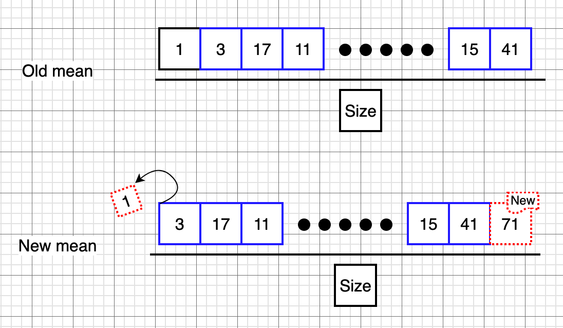
The idea of the incremental approach is relevantly easy to understand. Let’s have a look at the below illustration:

Illustration of appending new value into a rolling window.

When it comes to calculating the mean, we sum up all the elements in the queue and divide it by the length of the queue. As you can see, once you adding new value into the 22-day SMA rolling window, the numbers in the queue will mostly remain the same except the oldest value and the newest value. Therefore, all we need to do is take these two values into account and update the summation accordingly instead of looping through all the numbers in the queue.

$$\text{New mean} = \frac{\text{summation} + \text{new value} - \text{old value}}{\text{length of queue}}$$

Simply by applying this formula, we reduce the execution time down to 13ms.

for _ in new_dataset:
    new_value = _
    old_value = queue[0]
    queue.append(new_value)
    summation = summation + new_value - old_value
    m_queue_2.append(summation/len(queue))

# => Last executed at 2024-12-16 12:12:20 in 13ms

Now let’s use the below code to compare the results from both approaches.

pd.DataFrame([m_queue, m_queue_2]).T.rename(columns={0:'traditional', 1:'incremental'}).plot()

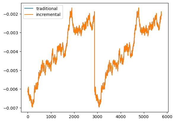
The mean values calculated with both traditional and incremental approaches

See! The incremental approach is giving the same results as the traditional approach, but use less time than the traditional approach does.

Variance & Standard Deviation

Now comes to the variance and standard deviation. The formula is as follows:

$$\begin{aligned}&\text{variance} &= \frac{\sum\limits_{i=1}^{n} (x_i - \bar{x})^2}{n}\\&\text{standard deviation} &= \sqrt{\text{variance}}\end{aligned}$$

Again, let’s start with initializing the queue and the lists that are needed to start the experiments:

queue = init_queue()
m_queue = m_queue_2 = list()

The traditional Approach

Below is the approach that everyone would do to calculate the variance and standard deviation:

for _ in new_dataset:
    new_value = _
    queue.append(new_value)
    m_queue.append(stdev(queue))

# => Last executed at 2024-12-17 00:50:27 in 2m 26.64s

This time, it cost 2m 26.64s to finish calculating 2880 times. It is apparently way slower than the mean calculation. As we all know, to calculate the variance and the standard deviation, we need to calculate the mean and then calculate the summation of the square of the difference between each data point and the mean. So the time complexity of calculating the variance and standard deviation is $O(n^2)$, meaning costing more time than the mean calculation.

The Incremental Approach

The incremental approach is a little bit more complicated than the mean calculation. We need to keep track of the summation of the queue, the mean of the queue, and the variance of the queue. This method is called the Welford’s Weighted incremental algorithm. You can also refer to this post for how to derive the formula using the very basic algebra. According to the formula, we can easily reduce the complexity from $O(n^2)$ to $O(n)$.

Again, let’s start with the initialization of the queue and the lists that are needed to start the experiments. But this time, we will calculate the summation, mean, and variance of the queue to conduct the following calculation.

queue = init_queue()
summation = sum(queue)
mean = summation / len(queue)
variance = sum([(x-mean)**2 for x in queue]) / len(queue)

Now, according to this post, we will simplify the formula to

$$\text{new variance} = \frac{\text{length of the queue} * \text{old variance} + (\text{new value}-\text{old value}) * (\text{new value} - \text{new mean} + \text{old value} - \text{old mean})}{\text{len of the queue}}$$

for _ in new_dataset:
    old_value = queue[0]
    new_value = _

    old_sum = summation
    new_sum = summation + new_value - old_value

    old_mean = summation/len(queue)
    new_mean = (summation + new_value - old_value)/len(queue)

    old_variance = variance
    new_variance = (len(queue)*old_variance + (new_value - old_value) * (new_value - new_mean + old_value - old_mean))/len(queue)

    queue.append(new_value)
    m_queue_2.append(sqrt(new_variance))

    # Update the summation,
    summation = new_sum
    variance = new_variance

# => Last executed at 2024-12-17 01:00:10 in 14ms

Hey, we greatly reduce the execution time needed from 2m 26.64s to 14ms. Last thing we need to do, is to examine the results from both approaches.

pd.DataFrame([m_queue, m_queue_2]).T.rename(columns={0:'traditional', 1:'incremental'}).plot()

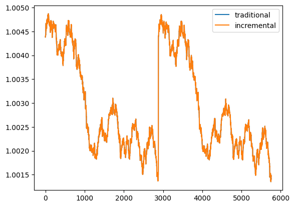
The mean values calculated with both traditional and incremental approaches

Great! The incremental approach is giving the same results as the traditional approach, but use less time than the traditional approach does. This is the power of incremental approach!

Take away

This is the power of math! If you follow the steps in the post to derive the formula, you will find that the formula is quite simple. However, by simply applying the formulas to the calculation, you’ll find out it saves you not just the time to calculate the variance and standard deviation, but also the memory space when you want to deploy the algorithm in a production environment. Hence, when you are working on a project, always try to think about the math behind the algorithm.