
Cover image created by Copilot
The best ideas are often inspired by or adapted from the work of others. Likewise, profitable quantitative trading strategies are not necessarily original, but they can be generated by adding personal insights regarding the market or strategy itself. In this post, I’m going to introduce the process that I usually do when discovering a prospering trading strategy.
Become a Medium member to support me in writing more interesting articles. I’ll receive a small portion of your membership fee if you use the following link, at no extra cost to you.
If you enjoy reading this and my other articles, feel free to join Medium membership program to read more about Quantitative Trading Strategy.
Previous researches
- Optimize your MACD strategies with advanced indicators
- 【Pair Trading】 Complete Guide to Backtest Cointegration Pair Trading Strategy
- 【ML algo trading】 II - How to build a machine learning boilerplate?
Buy-on-Gap trading strategy
Strategy origin
First of all, we need to find a promising trading strategy either from gossip, posts in the forum, or even books. In this post, I’m going to use the buy-on-gap strategy that I’ve found in Ernest P. Chan‘s book “Algorithm Trading - Winning Strategies and Their Rationale”.
Introduction of the benchmark trading strategy
The buy-on-gap trading strategy is a popular trading technique that involves identifying price gaps and making trades based on the anticipated price action following the gap. Price gaps typically occur when the market opens or due to unexpected fundamental and technical events. These events usually trigger panic selling and cause a disproportional drop in price. Since price gaps tend to get filled after the panic selling is over, professional traders use these blank areas to find trading opportunities.

Panic selling created by Copilot
Platform
I’m using QuantConnect to backtest this strategy.
Backtest period
From 2020-12-27 to now.
Trading Frameworks and Trading Rules
QunatConnect separates the quantitative trading script into five different parts. Universe model is to select the desirable equities, bonds, futures, options, or ETFs that you would like to trade against. Alpha model is to monitor the status of each asset, and then emit the trading signals accordingly. You need to adopt the Portfolio Construction model when you would like to specify the weight of each desirable asset in your portfolio. The Risk Management model also monitors the custom risk level of each asset. The model will help dispose of your holding asset when a certain risk management threshold has been hit. Therefore, you can develop your own model and mismatch it with other models with minimum work.
Now, let’s have a look at the models we need to build to build this buy-on-gap trading strategy:
Universe model
In the book “Algorithm Trading - Winning Strategies and Their Rationale”, Ernest P. Chan didn’t specify any preference regarding the universe selection. Therefore, I just pick the constituent stocks of ETF SPY as the benchmark scenario. The SPY (SPDR S&P 500 ETF Trust) is an exchange-traded fund that tracks the performance of the S&P 500 index, which is a basket of the largest publicly traded companies in the United States. Therefore we save the effort to track and to exam which fundamentals of each stock/company and hence select over 500 stocks.
Alpha model
First of all, we need to set up our trading rules for the Alpha Model to monitor the market data and generate trading signals. The alpha trading signals generated essentially indicate that there are certain assets that we monitor in the Universe Model that have passed the predefined trading rules. Therefore, we can consider these assets as the constituents of our portfolio. Here are the trading signals generation rules:
- Select all stocks near the market open whose returns from their previous day’s lows to today’s opens are lower than on standard deviation. The standard deviation is computed using the daily close-to-close returns of the last 90 days. These are the stocks that ‘gapped down’
- Narrow down this list of stocks by requiring their open prices to be higher than the 20-day moving average of the closing prices
- Buy the 10 stocks within this list that have the lowest returns from their previous day’s lows. If the list has fewer than 10 stocks, they buy the entire list
- Liquidate all positions at the market close
I intentionally skip rule No.2 as the benchmark strategy to gain a full picture of this buy-on-gap trading strategy. Therefore, we can build our Alpha Model based on the above trading rules:
Portfolio Construction model
After the trading signals are generated, we must determine the percentage of these assets to be included in our portfolio. According to trading rule No. 3 above, we will allocate the capital evenly to each asset candidate. If we have less than 10 signals generated in one day, then we still allocate all the capital to these assets evenly.
Risk Management Model
The Risk Management Model by meaning is a model used to manage the risk level of each single asset. This is also where to implement the stop loss and stop gain mechanism. Even though this mechanism was not mentioned anywhere in the trading rules from the book, I believe it can be one of the variations of our trading scenarios. In this simple setup, we define the stop gain rate to be 2% and the stop loss rate to be 1%, meaning we will sell specific holding assets once the daily return is above 2% or below 1%.
Main Script
Lastly, we’re going to use main.py to include all the sub-models that we created so far. Noted that we don’t include the Risk Model yet in the backtest scenario of our trading algorithm.
Plain Vanilla Scenario Result
| Strategy | Total Return | Annualized Return | Total Trades | Win Rate | Sharpe Ratio | Drawdown | Annual Variance | Expectancy |
|---|---|---|---|---|---|---|---|---|
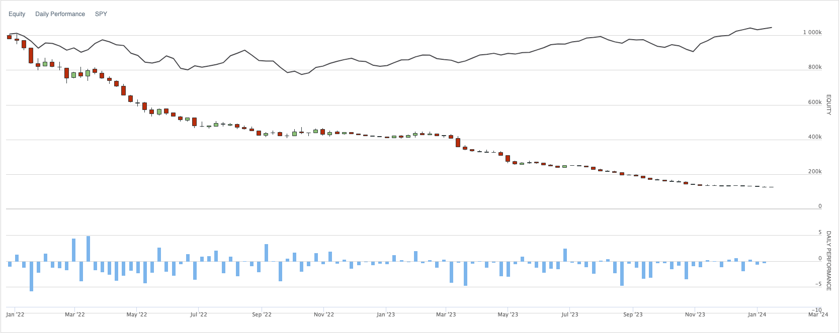
| Plain Vanilla | -83.389% | -57.726% | 3366 | 47% | -0.826 | 85.300% | 0.254 | -0.128 |
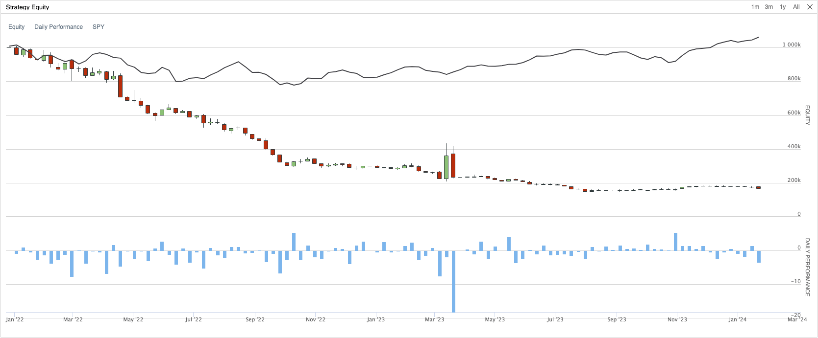
Backtest results of plain vanilla buy-on-gap strategy
Sadly, the course of true love never did run smooth. The backtest result of our plain vanilla buy-on-gap trading strategy is not as good as suggested in the book, and it’s even cost our entire initial capital. Thanks to the author of this article, that the author had kind of explaining the trend that this strategy seems to have been ineffective since 2008 and has become worse since 2018. That also gives us the incentives to turn this around.
Now the Show Begins
As said, we’re not going to stop right here. Now let’s try to find out some other hidden patterns from the different aspects of fundamental methodologies.
Enhance the strength of the signal (Add sma-20 to confirm the trend)
As the first variation, let’s add back the trading rule No.2 Narrow down this list of stocks by requiring their open prices to be higher than the 20-day simple moving average of the closing prices to see how it impacts the buy-on-gap trading strategy.
1 | """In CustomDiversifiedAlphaModel.py""" |
| Strategy | Total Return | Annualized Return | Total Trades | Win Rate | Sharpe Ratio | Drawdown | Annual Variance | Expectancy |
|---|---|---|---|---|---|---|---|---|
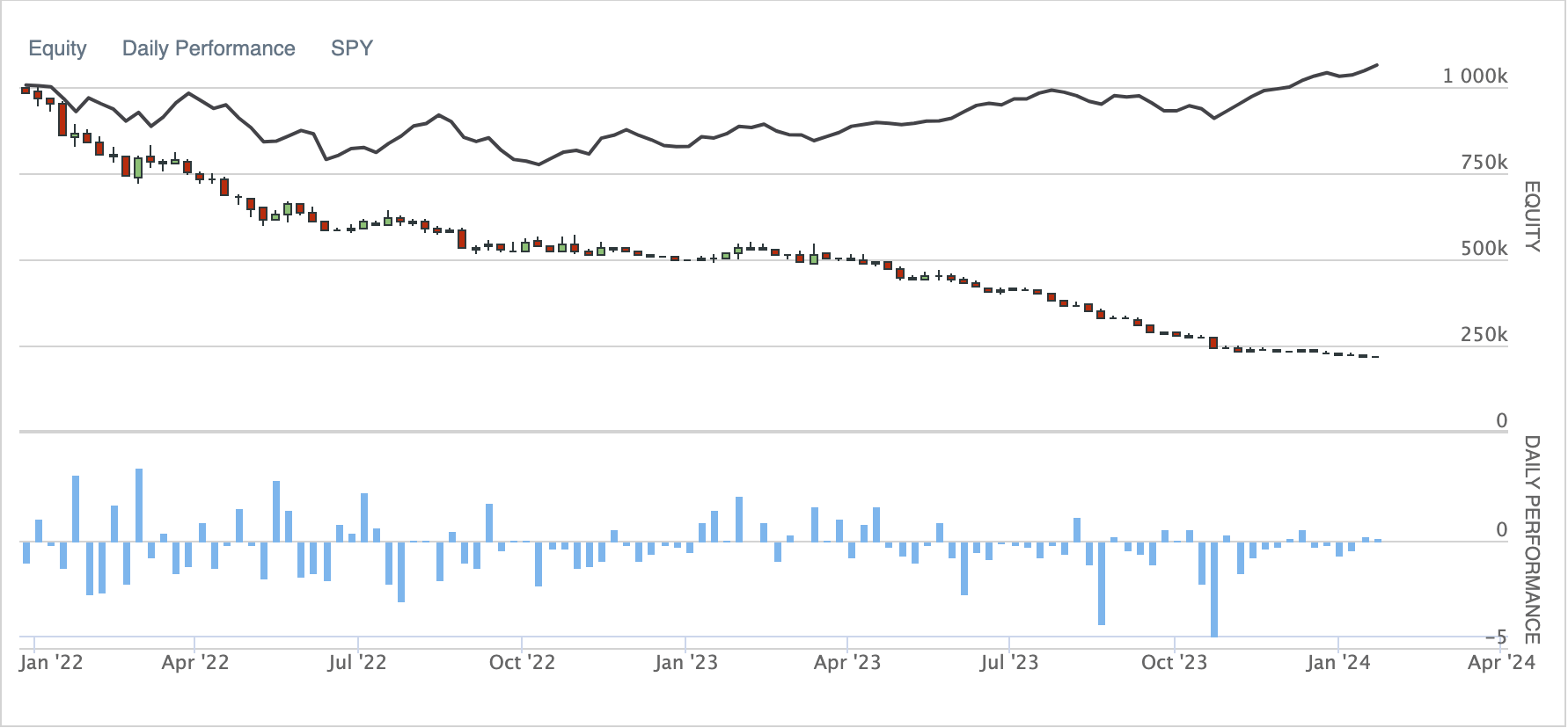
| Plain Vanilla with sma20 | -5.35% | -2.604% | 604 | 46% | -0.249 | 21.4% | 0.027 | -0.007 |
Backtest results of plain vanilla buy-on-gap strategy plus sma20 of the closing price
Even though we have not yet turned this trading strategy into a profitable one, the loss of our portfolio has significantly reduced. However, once you lay your eyes on the report, the first thing you’re going to notice is the number of total trades which has dropped from 3000+ to 600 trades within our trading periods. Therefore, trading rule No. 2 served the purpose of filtering out those poisonous trades but failed to increase the win rate.
Other than the insights drawn above, the intention of adding more rules to further confirm the trend is considered as overfitting your strategy to the past market data. Therefore, I would not recommend applying too many additional rules to your trading strategy.
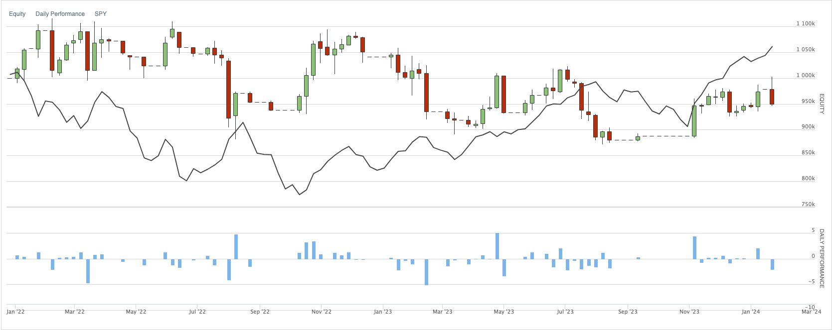
Weighting method: All-in or equal-weighted
As Ernest P. Chan said in the book, this trading strategy has a relatively small capacity compared to others, and only a couple of signals or no signals are generated each day. This also means that it is very likely that our capital will be allocated to one individual stock when there’s only one signal was generated on that particular day. Once this is a bad trade, we’ll suffer a devastating loss. To reduce the risk and the potential damage caused by this worst-case scenario, we can apply the equal-weighted method to diversify this risk.
1 | """In CustomPortfolioConstructionModel.py""" |
| Strategy | Total Return | Annualized Return | Total Trades | Win Rate | Sharpe Ratio | Drawdown | Annual Variance | Expectancy |
|---|---|---|---|---|---|---|---|---|
| Equal-weighted | -38.91% | -21.048% | 3364 | 47% | -1.189 | 45.50% | 0.022 | -0.101 |
| Equal-weighted with sma20 | 0.535% | 0.256% | 604 | 46% | -0.967 | 5.80% | 0.001 | 0.012 |
Backtest results of buy-on-gap strategy applying the equal-weighted method
Plus additional 20-day Simple Moving Average
The results of applying the equal-weighted method are phenomenal! This tells us that with the right tools, we still can turn the dreadful situation around. Of course, with the overall performance and the fact that the win rate is still lower than 50%, this variation still can’t qualify as a good qualitative trading strategy.
Mean-Reversion V.S. Momentum
Mean-reversion and momentum strategies are essentially two sides of the same coin. When the stock price of a specific stock reaches a certain point (either upward or downward), the believer of the mean-reversion theory would expect the stock price to return to equilibrium. On the other hand, the followers of the market momentum are convinced that the possibility of the stock price would ride on the trend and continue to either grow or drop when that certain point is passed. Since the buy-on-gap trading strategy is a strategy that expects the stock price to revert to its normal level after the previous overnight trading anomaly, we can also hold the contrary point of view saying that the trend will continue after the anomaly.
1 | """In CustomDiversifiedAlphaModel.py""" |
| Strategy | Total Return | Annualized Return | Total Trades | Win Rate | Sharpe Ratio | Drawdown | Annual Variance | Expectancy |
|---|---|---|---|---|---|---|---|---|
| Momentum | -87.263% | -63.248% | 10001 | 43% | -2.26 | 87.3% | 0.053 | -0.189 |
| Momentum with sma20 | -78.422% | -52.704% | 9747 | 42% | -2.192 | 78.40% | 0.037 | -0.164 |
Backtest results of buy-on-gap strategy as momentum trading strategy
Backtest results of momentum buy-on-gap strategy plus sma20 of closing price
Ok, our point of view does not hold. Turns out that there is no either mean-reversion or momentum DNA in the buy-on-gap trading strategy anymore. However, let us take a step back and see this chart from a different angle. Since this downward performance is an inevitable outcome, why don’t we change our trading direction to turn this situation “upside-down”?
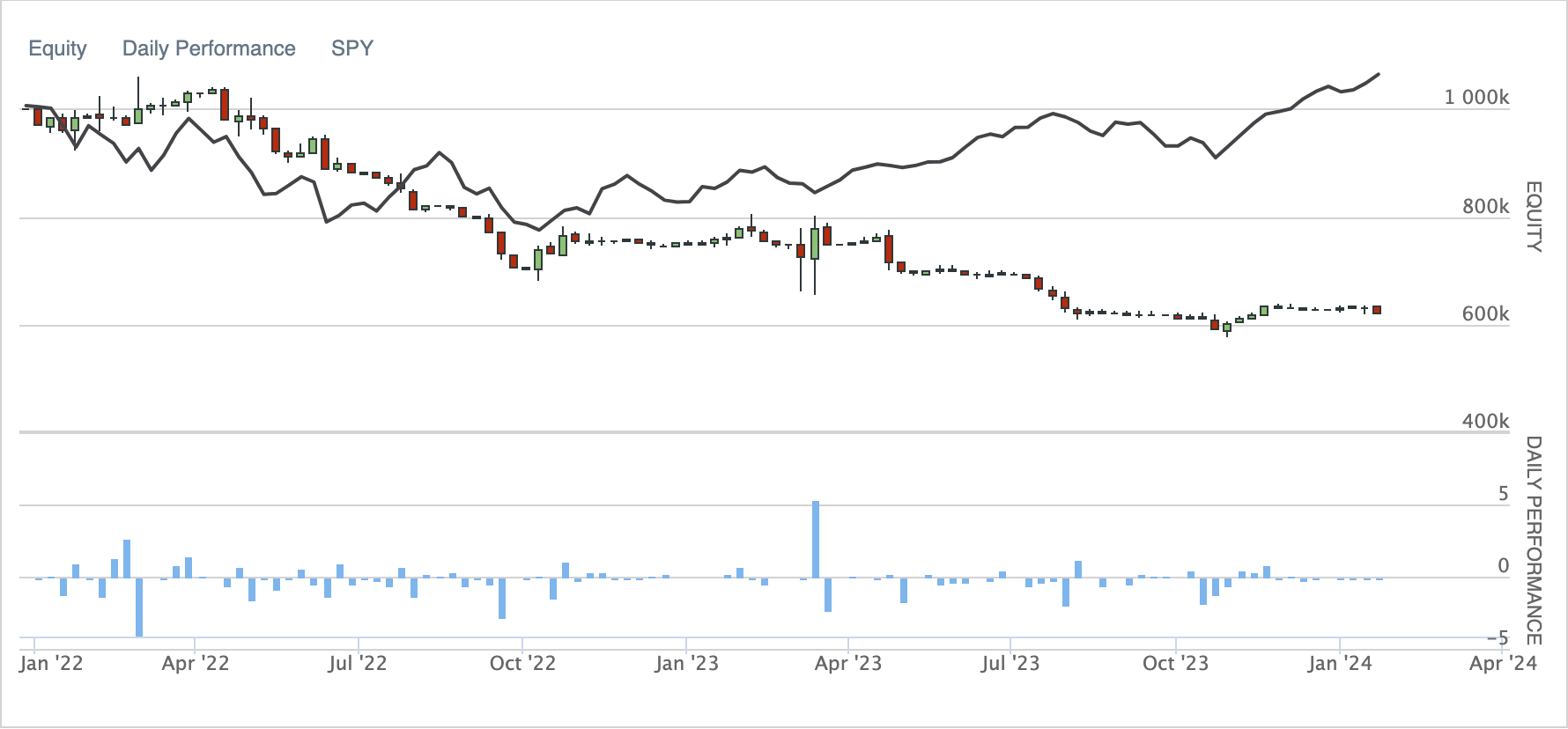
Long v.s. Short
The idea is relatively simple. Originally, we long a stock at \$10.00 and expected it to rise after the anomaly last night. Unfortunately, the thing went south and we got to sell it at \$9.5 before the market closed. Accumulating these constant losing trades cost us the capital of our portfolio. On the contrary, if we short a stock at \$10.00 and close it at \$9.5, wouldn’t the same scenario help us accumulate our fortune?
1 | """In CustomDiversifiedAlphaModel.py""" |
| Strategy | Total Return | Annualized Return | Total Trades | Win Rate | Sharpe Ratio | Drawdown | Annual Variance | Expectancy |
|---|---|---|---|---|---|---|---|---|
| Short trades | -77.69% | -51.181% | 3369 | 44% | -0.59 | 83.10% | 0.262 | -0.110 |
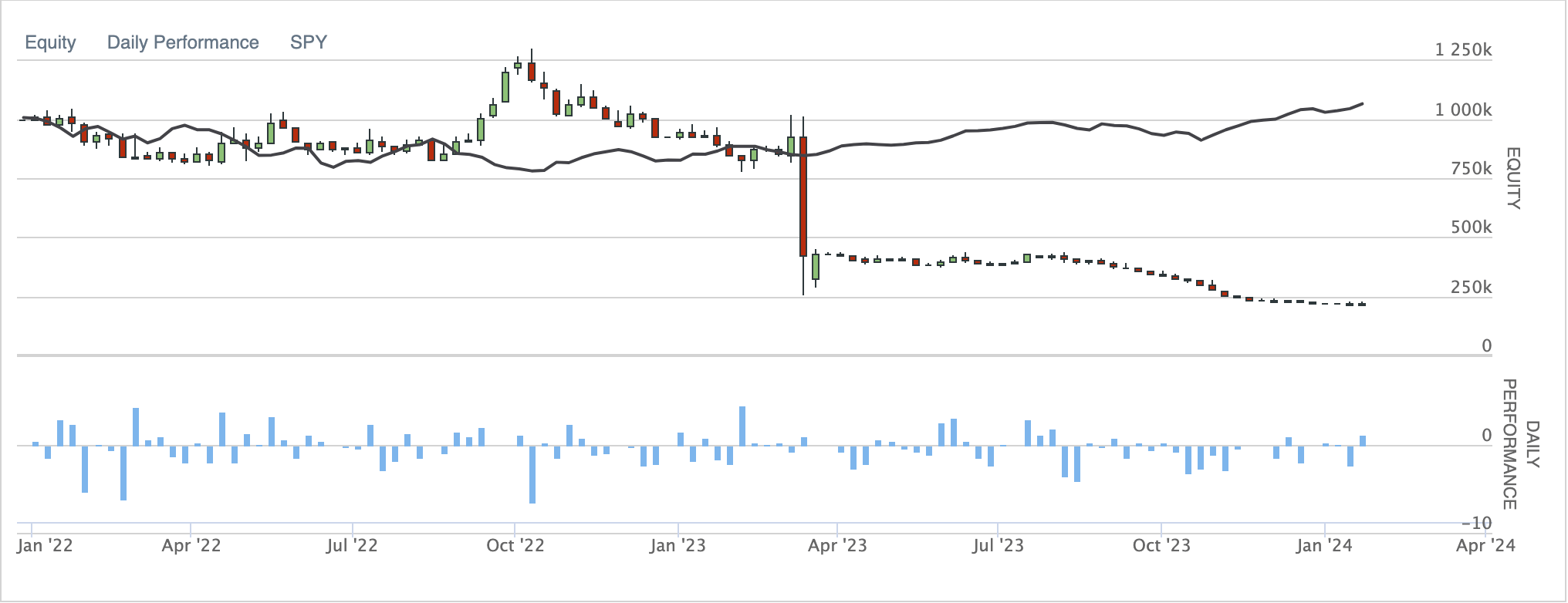
Backtest results when turning all the long trades into short trades
The first half of the backtest was quite inspiring to see that my point was proved, … until the long red bar popped in my face… I browsed through my transaction history, and I found out this spoilsport turns out to be FRC (First Republic Bank). If we’re able to use sentiment analysis as suggested in Sentiment Analysis lesson 101 and hands-on practice session, we might be able to filter out this poisonous stock and further avoid significant loss in our portfolio.
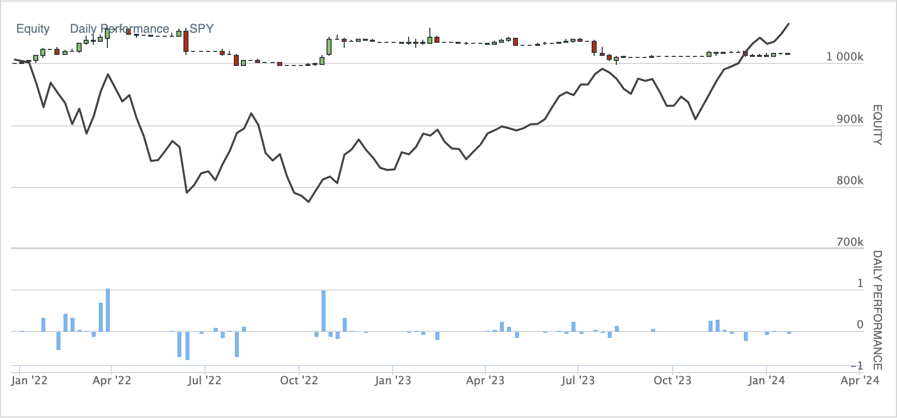
Stop loss and stop gain
The initiative of adopting the stop loss and stop gain in the buy-on-gap trading strategy is that, even though the price will eventually revert to the original level before the anomaly as we believed, the momentum of that reversion will dwindle at one point and then in the end price will start to fall before the market close. Therefore, adding the stop gain and stop loss will help us harvest the crop before the upward momentum is depleted.
1 | """In main.py""" |
| Strategy | Total Return | Annualized Return | Total Trades | Win Rate | Sharpe Ratio | Drawdown | Annual Variance | Expectancy |
|---|---|---|---|---|---|---|---|---|
| Short trades | -85.27% | -59.970% | 3367 | 29% | -3.695 | 85.40% | 0.018 | -0.328 |
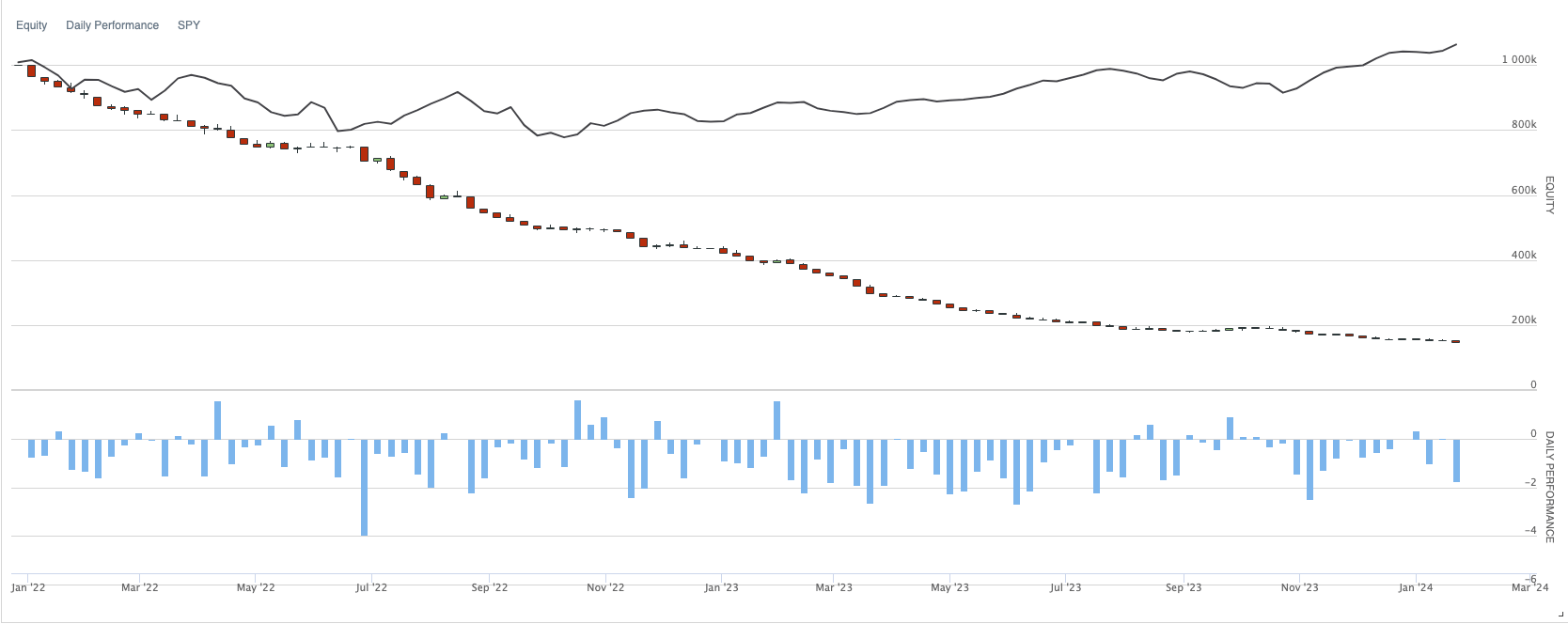
Backtest results when applying stop gain and stop loss
There are a few things that I’ve found after applying the stop gain and stop loss:
- After adding the stop loss and stop gain, I found out that there were a lot of stocks were sold right after our long positions were opened.
- The win rate dropped considerably from ~46% to 29%.
The above two clues give us a premature idea that the price-upward momentum happens sometime after the market opens instead of the time that the market just opens. Therefore we had another idea to discover the pattern of the stock price movement after the overnight anomaly, which I’m not going to further develop in this scenario here.
Others variations
There are some more variations suggested in the book Algorithmic Trading - Winning Strategies and Their Rationale by E.P. Chan plus some ideas we discovered while conducting the backtest above:
- Turning it into a market-neutral - long-short strategy
- Turning the strategy into a sector-neutral trading strategy so that it is less concentrated in the same industry
- Adopt machine learning technique to better identify the trading signal (Reference: 【Momentum Trading】Use machine learning to boost your day trading skill - meta-labeling)
- Adopt alternative data to develop brand-new insights. (Reference: Sentiment analysis lesson 101 and hands-on practice session)
Conclusion
In this post, we have explored different aspects and angles to approach this classic trading strategy, trying to revive this strategy into a profitable one. Even though the backtests we conducted didn’t present a positive enough Sharpe Ratio to put this trading strategy forward, we did develop a few interesting insights that are worth further looking into. In the end, let’s keep in mind that there are some limitations mentioned in E.P. Chan’s book:
- Drops caused by negative news are less likely to revert.
- This strategy can succeed in a news-heavy environment where traditional intraday stock-pair trading will likely fail.
- This strategy might not have a large capacity
- A pitfall of it is using consolidated prices v.s. using primary exchange prices.
Feel free to let me know how you like this subject. Cheers,
Reference
- Algorithmic Trading - Winning Strategies and Their Rationale by E.P. Chan
- QuantConnect Official API Document
- Buy on gap strategy and its performance over time