
Photo by Aaron Burden on Unsplash
In the last post, we learned the basics of performing the pair trading strategy and using cointegration as a method to identify the potential tradable stocks pair. All the theories and the math formulas are so seemingly promising and convincing enough for us to believe it’s a profitable and stable trading strategy. But is it? In order to test and check the profitability and effectiveness of this strategy, we need to backtest this trading strategy to simulate real-world scenarios.
Become a Medium member to continue learning without limits. I’ll receive a small portion of your membership fee if you use the following link, at no extra cost to you.
If you enjoy reading this and my other articles, feel free to join Medium membership program to read more about Quantitative Trading Strategy.
Previous researches
Recap
Let’s pick up where we left off.
In the last post, we spent time explaining the basic concepts of cointegration pair trading strategy such as what cointegration means, the meaning of stationary, and how we profit from these concepts. We chose Engle-Granger 2-step approach as a method to inspect the level of cointegration between two time series. Once we are able to find the stock pairs that have higher probabilities to stay cointegrated, then we can start monitoring the co-movement of their price and make trades when the pairs are temporarily not cointegrated.
We’ve also revealed the preliminary trading rules of the cointegration pair trading strategy. We
- Open a long position if the current spread is smaller than the mean of the spread $\mu - threshold * \sigma$
- Close a long position if the current spread is bigger than the mean of the spread $\mu$
- Open a short position if the current spread is bigger than the mean of the spread $\mu + threshold * \sigma$
- Close a short position if the current spread is smaller than the mean of the spread $\mu$
Where
- The mean of the residuals ($\mu$) as the benchmark line in our residual observation
- The standard deviation of the residuals ($\sigma$) to calculate the trigger line in our residual observation
- The threshold would be 2.32, indicating a 99% of the confidence level
Even if we’ve done a lot of research to learn as much as we can about the pair trading method, there are some factors we can’t avoid in real-life settings. As a result, this is where backtesting comes into play. Conducting a successful backtest would mean a lot to simulate what is going to happen if you throw your trading strategy into the wild and unpredictable stock market.
Build our trading rules
To conduct a backtest, we first need to set up the ground for this pair trading strategy. Here are a few trading rules that I have put together.
Trading pair formation
- Selecting around 500 stocks based on their company financial fundamental data to find the companies that are stable and relatively financially healthy.
- Obtaining the daily close price from the past two years for every stock that we picked
- Using the
scipy.stats.pearsonr(Series_A, Series_B)to calculate the Pearson correlation, and chose the stock pairs whose correlation value is bigger than0.9and the p-value is smaller than0.05 - Using the Engle-Granger 2-step approach to examine every existing pair
- Using
sm.OLS(Series_B as y, Series_A as x).fit()to get the beta, intercept, and residual of each pair - Using
statsmodels.tsa.stattools.adfuller(model.resid, autolag = 'BIC')to evaluate the level of stationary of the residual of this pair - Eliminating the stock pairs whose cointegration p-value is bigger than
0.05, shows the stationary property is less significant.
- Using
- Lastly, we sort these pairs by their cointegration p-value, the smaller the better.
- We repeat this process every month in order to closely follow the cointegration status of the potentially tradable stock pairs.
Monitoring and trading
Since the pairs have been filtered and sorted by their level of correlation and cointegration, we consider these stock pairs to be our stock pair universe. As the methodology mentioned in the previous post, we are already using the data of the past two years to build the upper and lower bands. There are more details to be defined in order to complete our trading strategy.
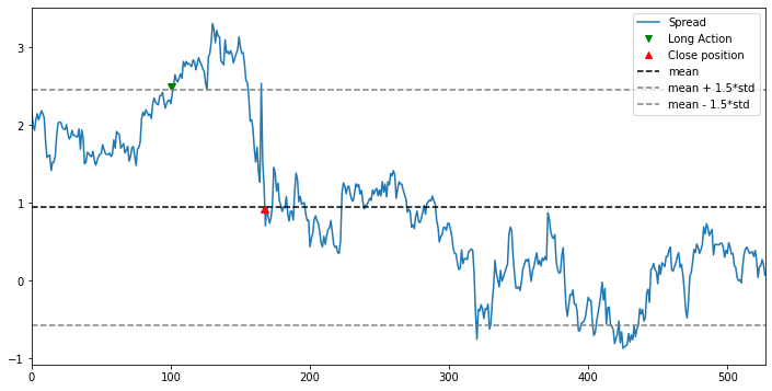
The upper and lower bands built from the residual of the OLS results
Observing frequency
We examine the status of the pairs in our observing universe and the pairs that we already traded for every 15 minutes. Since we’re using the daily close price to form the trading pairs and to trade accordingly, I presume that 15 minutes would be an ideal interval to inspect the status of the pairs.
Enter and exit signals
The basic idea of signal generation has been stated in the Recap section above, so I won’t waste any of your time and rewrite them here again.
Stop loss and stop gain
In the post of 【Momentum Trading】Use machine learning to boost your day trading skill - meta-labeling, we have learned the idea of using the Triple Barrier Method (TBM) to control our gain/loss ratio. In this pair trading strategy, I’m using 2:1 as our gain/loss ratio. This 2:1 ratio essentially indicates that we will be able to tolerate 50% of our expected gain as our maximum loss per trade. For example, in our trading rules, we will close the pairs for those pairs whose residuals ($\mu$) return to the level of 0, meaning the stop gain would be 2.32 as we exit the trades when the residual is back to the level of 0. Then we define our stop loss to be at the level of 2.32 + 2 (2.32 - 0) / 2 = 4.64 and exit our trade at it in order to prevent greater loss when both stock prices further deviate.
As the ground rules have been set up to implement our trading strategy, I’m going to run the first round of backtest to see how it performs and to check the profitability of this strategy.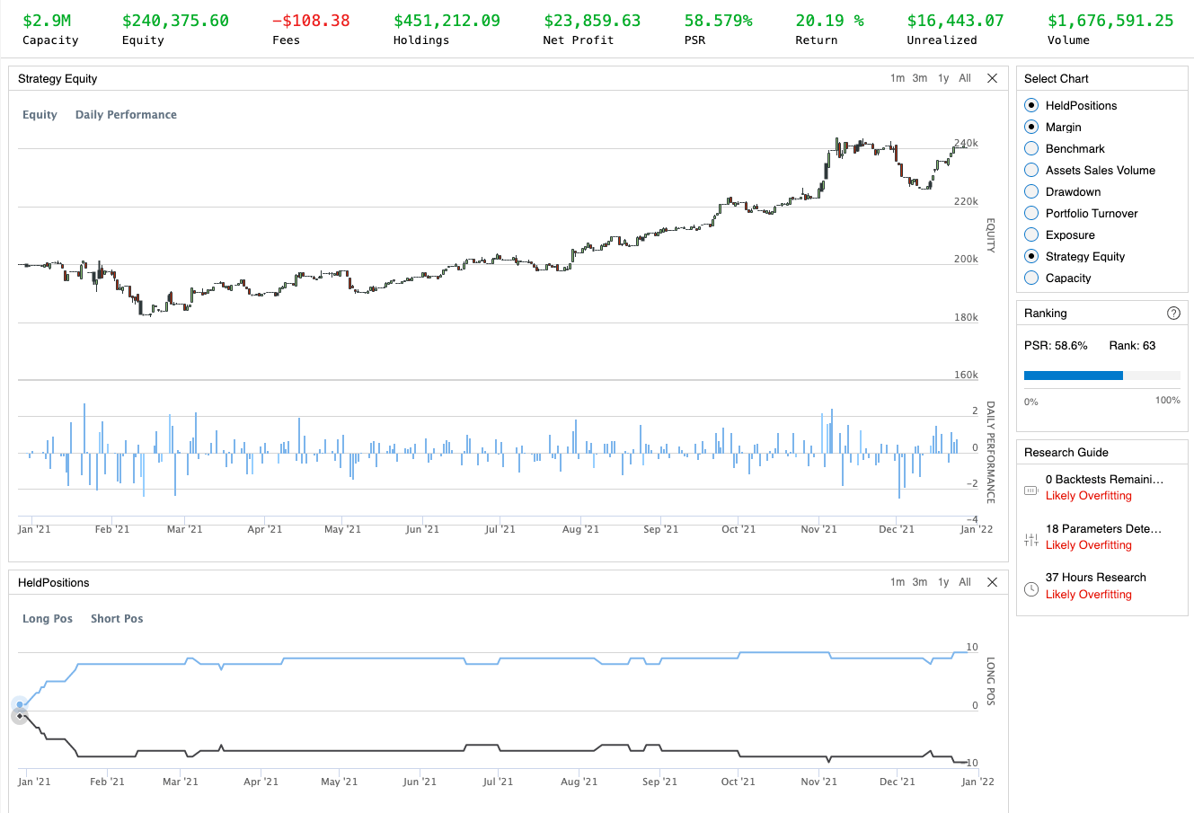
First-round backtest of the pair trading strategy
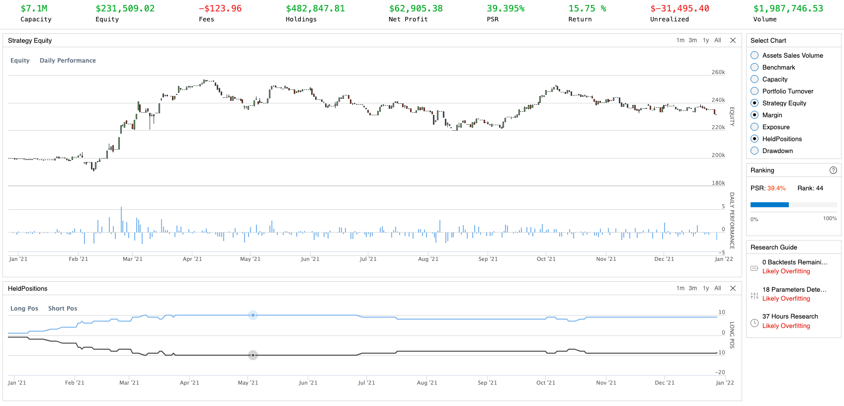
Wow! At first glance, the performance was quite impressive and satisfying. However, if we get a closer look, some illogical mistakes hide behind this backtest result. In the bottom chart HeldPositions, the number of long positions and the number of short positions should equal all the time, as we trade pairs including one long stock and one short stock. Therefore, in the red circle, you can tell the number of one side was decreased and the other side wasn’t. This would leave our portfolio exposed to risk as our positions were not hedged properly, increasing the odds to lose money on such an anomaly in our portfolio.
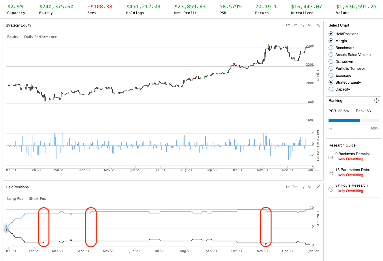
Red circles indicate weird things happened in our trading activities
Several scenarios we need to consider and address
After looking into the log message in the tested backtest, several loopholes can be found and concluded in my trading strategy: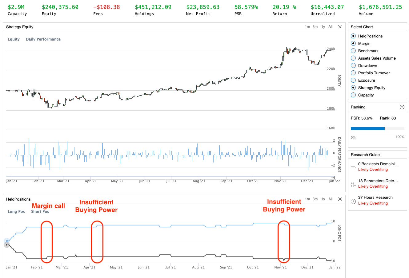
Incorrect trading activities that need to be taken care of properly
Hazard 1: Margin call
According to the trading log message, the first red circle was due to the margin call getting executed to recover the remaining margin in your margin account. In order to trade stock options or to short-sell assets, you are required by brokers to retain the investor’s equity above a certain percentage so that you demonstrate your capability to repay the potential loss of your current investment. Once such a loss occurs and your equity falls under this percentage, you will receive this margin call notice from the broker that requires you to sell a part of your investment and turn it into cash to raise the percentage of equity.
In our backtest, the stock price of TSLA has declined drastically which brought the percentage of equity below that percentage, that’s why we were forced to sell any investment and turn it into cash. The point being, that we don’t want to sell ANY asset in our portfolio. Instead, we need to make sure we sell a pair of assets to remain our market neutrality. In the meantime, we also need to decide which pair to be liquidated that has the least impact on our trading strategy. In the paper An Anatomy of Pairs Trading: The Role of Idiosyncratic News, Common Information and Liquidity, the experiments demonstrate that the probabilities and profitability of the pair start to increase day by day since the deviation has been detected, and then it will start to decline since reaching the top performance on day six. Therefore, I made an assumption that the longer a pair was held, the lower probability for this pair to be profitable. So we need to sell the pair that we hold the longest when the margin call occurs.
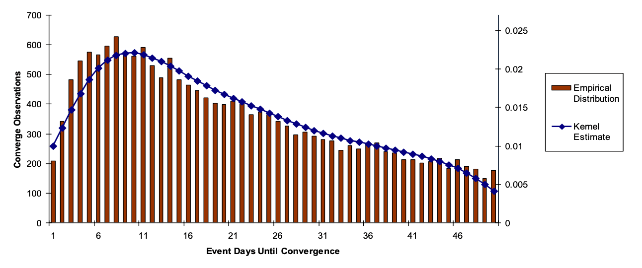
The profitability dwindles as the day pass
Hazard 2: Fails to place two orders (one long and one short) simultaneously
The other two incidents in our HeldPositions plot are referring to Insufficient Buying Power. Buying power is a concept that is quite easy to understand but is relatively complex to calculate. According to Understanding IB Margin Webinar Notes, the buying power can be defined as follow:
Buying Power
Is the value of securities you can purchase without depositing additional funds. In cash accounts this is the settled cash. In a margin account, buying power is increased through the use of leverage using cash and the value of held stock as collateral. The amount of leverage depends upon whether you have a Reg. T Margin or Portfolio Margin account. Active traders can take advantage of reduced intraday margin for securities – generally 25% of the long stock value. But keep in mind this requirement reverts to the Reg T 50% of stock value to hold overnight.
$\text{Cash Account Buying Power} = Min(\text{Equity with Loan Value, Previous Day Equity with Loan Value}) –\text{Initial Margin}$
$\text{Margin Account Buying Power} = \text{Cash Account Buying Power} * \text{Leverage Ratio}$Formulas to calculate the Buying Power
Given the buying power as the limitation of placing orders with the margin account, we will face the scenario that one of the orders in the pair is successfully executed but the other order failed to be executed because the buying power of the day is insufficient. Unfortunately, QuantConnect doesn’t provide a function to check the current buying power in real-time. Therefore, we also need to come up with a solution to remedy this problem.
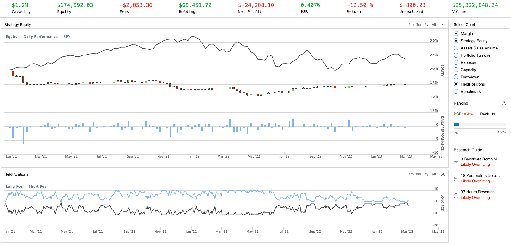
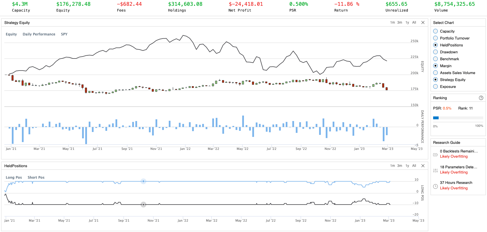
Backtest result after fixing the loopholes found
We have spotted two different potential scenarios that might endanger the profitability of our trading strategy, and we have successfully addressed them in a more theoretically trustworthy method. Looking back to the number of long positions and short positions in the plot HeldPositions are the same at all times. Now we can move on to the last part of the backtest.
Backtest
Even if we have successfully replicated the pair trading technique that has been profitable for the past two years, a single backtest cannot guarantee that this backtest will perform similarly in the real world. However, we may employ this backtest as a research tool to determine which parameters could potentially improve the win rate and Sharpe Ratio. This is so-called Hyperparameter Optimizing. In this section, I’m going to run backtest against several scenarios to answer the following questions:
- Should we use close price or log(close price) while calculating cointegration parameters and epsilon
- Does the profitability impact by the holding period as stated in An Anatomy of Pairs Trading: The Role of Idiosyncratic News, Common Information and Liquidity?
Therefore, I’m going to create eight scenarios usingprice/log(price)and close the pair trade when it’s been10/22/132/264 daysindicating we close the trade after it’s 10 days, one month, six months, and one year.
Furthermore, aside from the standard KPIs such as Total Return, Sharpe Ratio, and MaxDrawDown, other KPIs such as Win Rate will be incorrect because it is based on a single stock and always equals around 50%. Hence I wrote a script to process the order records into a pair-wise order record and visualize the pair-wise performance.
Platform
Backtest Periods
2020/12/27 - 2023/03/03
Backtest Universe
As stated in the section Pair formation
Backtest benchmark
SPDR S&P 500 ETF Trust (SPY)
Backtest Results
Strategy-wise performance
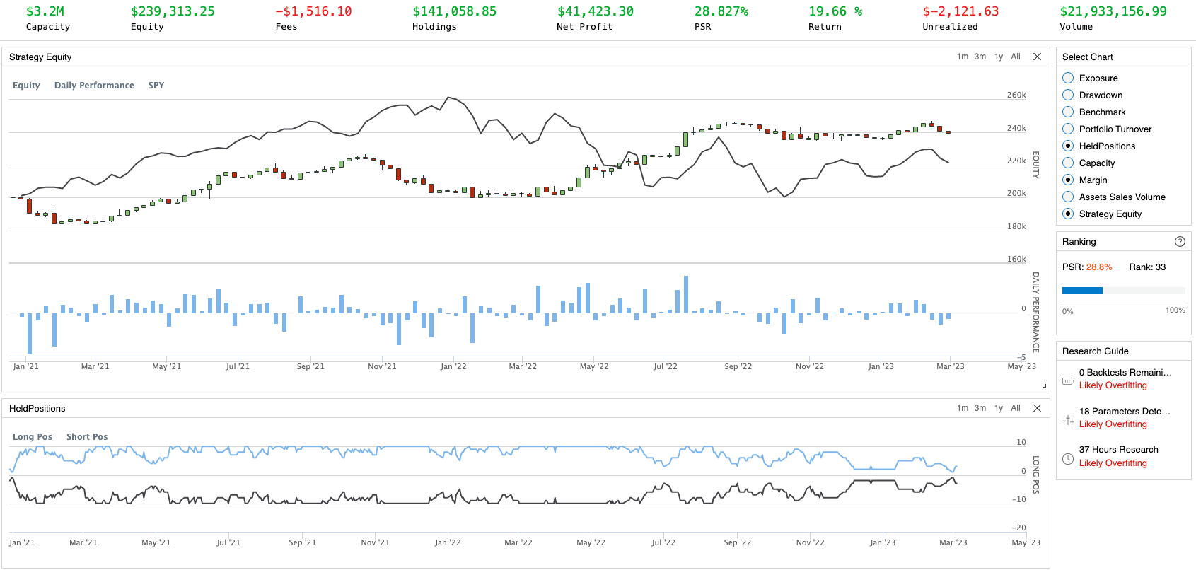
| Using close price | Using log(close price) | |
|---|---|---|
| Close after 10 days | 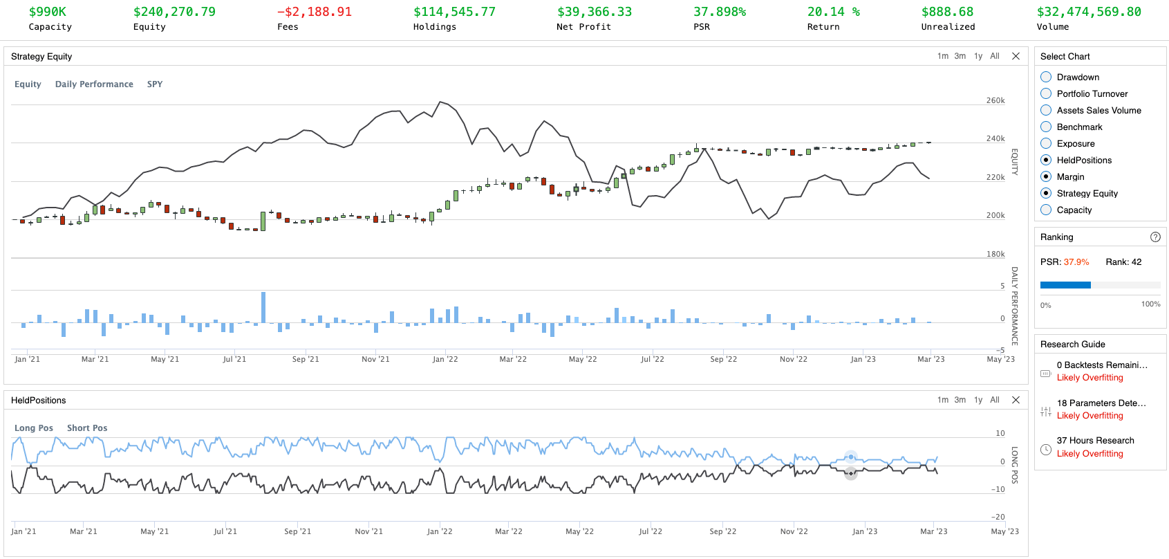 |
 |
| Close after one month | 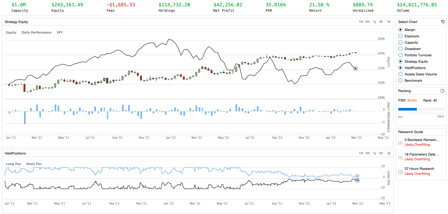 |
 |
| Close after six months | 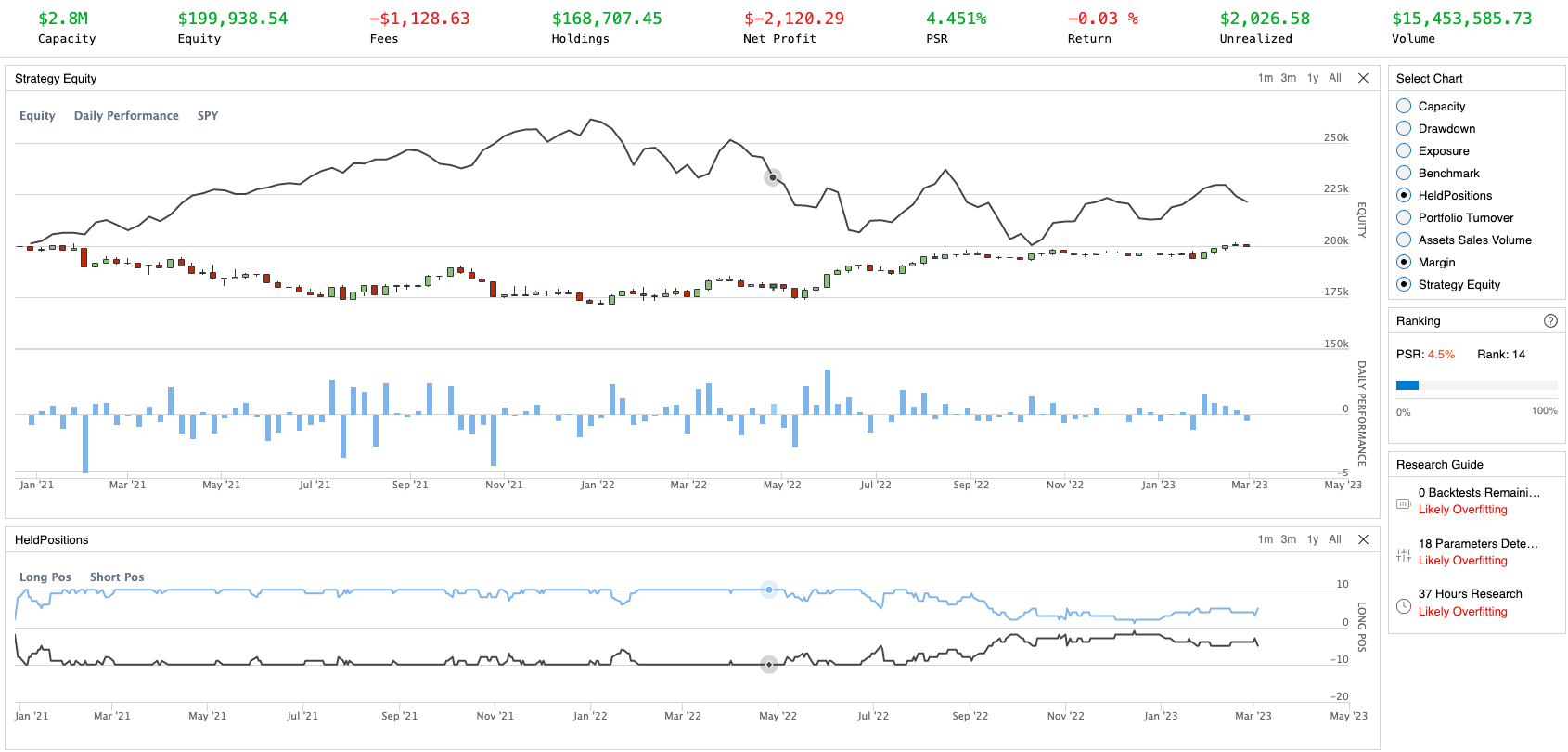 |
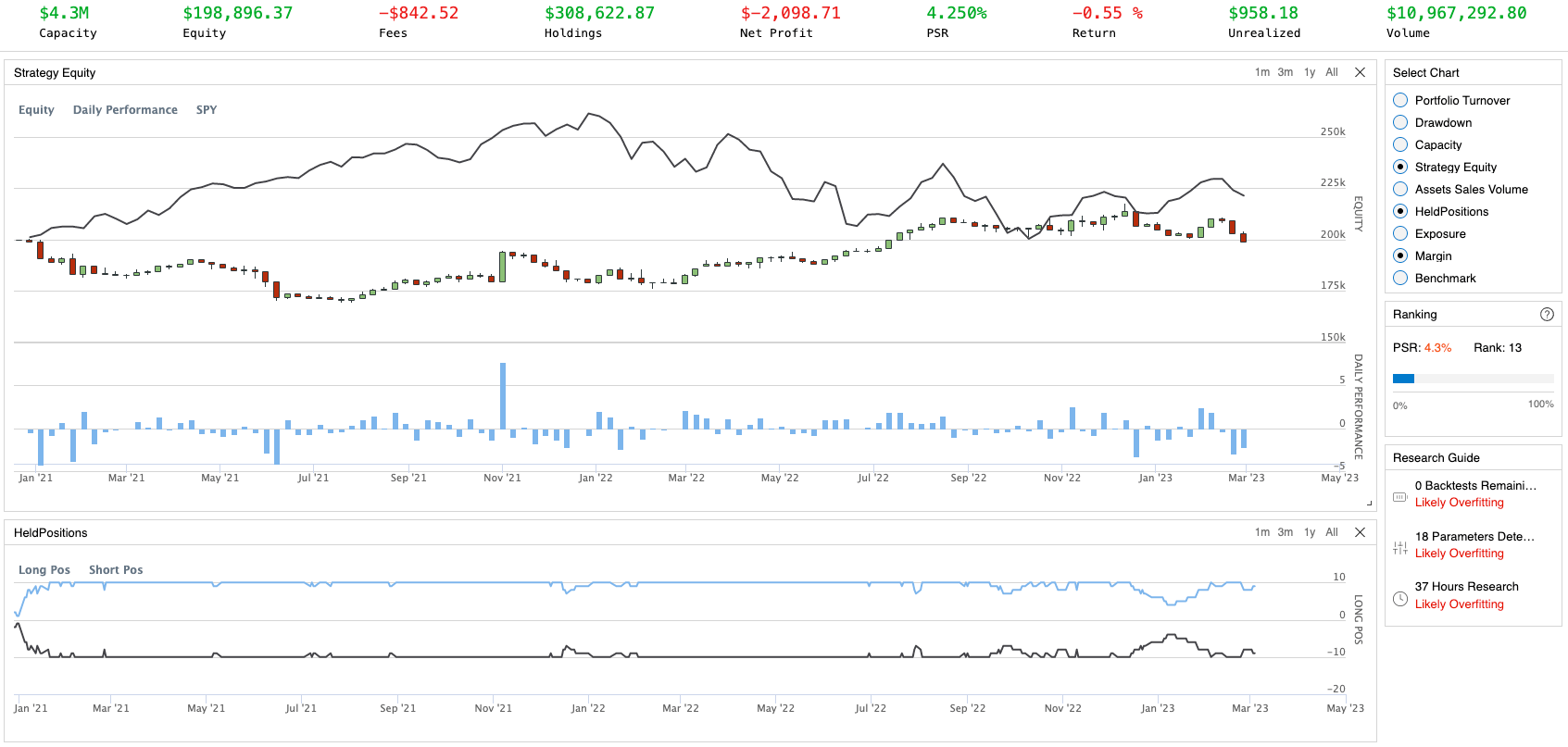 |
| Close after one year | 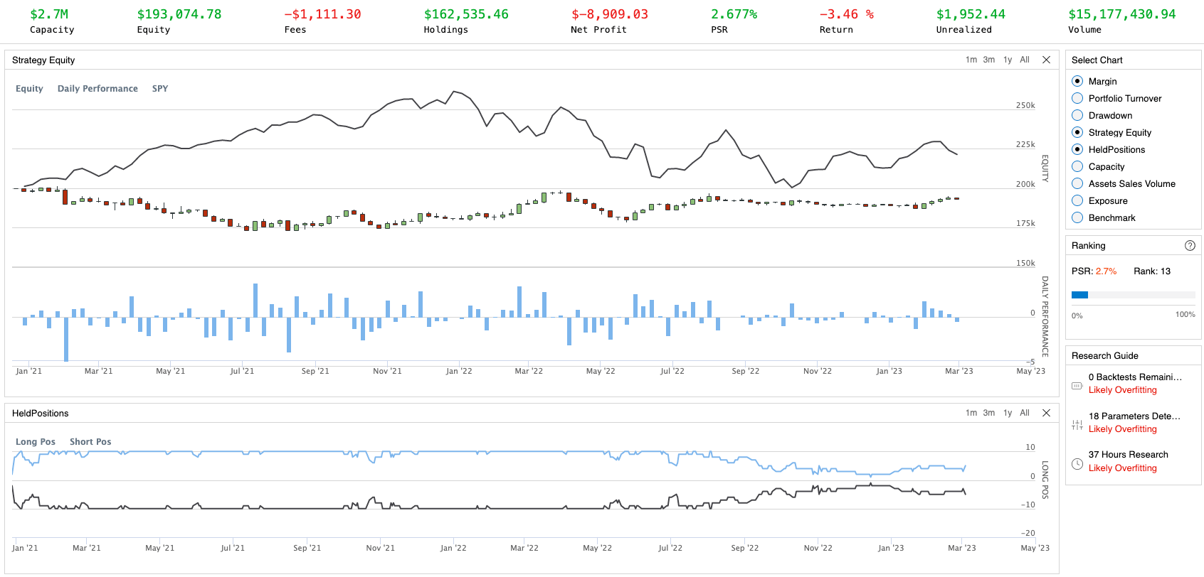 |
 |
Strategy-wise performance of every scenario
Once I put the backtest results altogether, it’s quite easy to notice that the performances of the pair trading strategy do conform to the curve as we see above but not exactly following the days in the plot. You can tell that the portfolio returns that close after six months and one year is comparatively lower than the portfolio returns that close after 10 days and one month. The scenarios that have the highest portfolio returns are all closing the trade after one month, no matter whether it’s using close price or log(close price).
On the other hand, the scenarios using close price don’t seem to have an obvious edge compared to the scenarios using log(close price). I guess we need some more parameters involved and more backtests to be performed in order to find out whether the difference exists.
Pair-wise performance
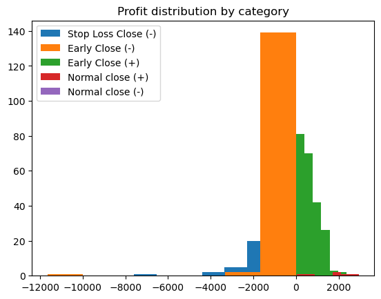
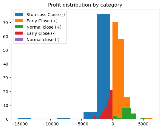
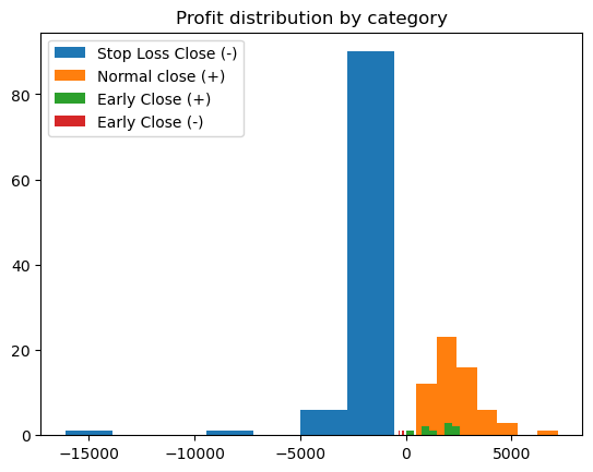
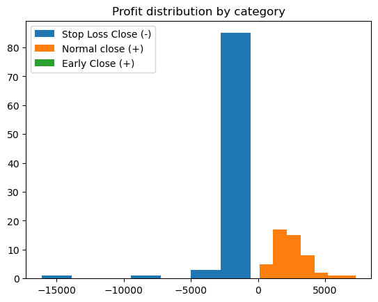
Before we shift our focus to this part, there are a few types of labels that I need to explain beforehand:
- Normal Close: This type of order is the order that received the sell signals before hitting the holding period limitation, the same as hitting the vertical time bar of the Triple Barrier Method (TBM) (see here for more details). In the most optimal case, we would like to see the more Normal Close orders the better, as they are the orders that follow the central idea of pair trading to produce positive profit via buying when two stock prices deviate and selling when two stock prices start to cointegrate.
- Early Close: This category represents the orders that are not yet received the sell signals but hit the vertical time bar. The Early Close orders are considered as their momentum/energy/tendency to converge are less stronger than they used to be, therefore we close them before they converge in exchange for other pairs that have higher chances to converge. They could be in the money or out of money while we close these Early Close orders and have higher uncertainty compared to normal close orders. We use
+to label this pair trading generate positive profit and-to label this trade’s profit as negative. - Stop Loss Close: These orders are closed because their epsilons are getting too big or too small, indicating the prices of the stocks in this pair are starting to further diverge. To avoid a huge loss, we close this type of order before we hit any other bands. We use
+to label this pair trading generate positive profit and-to label this trade’s profit as negative.
| Using close price | Using log(close price) | |
|---|---|---|
| Close after 10 days | 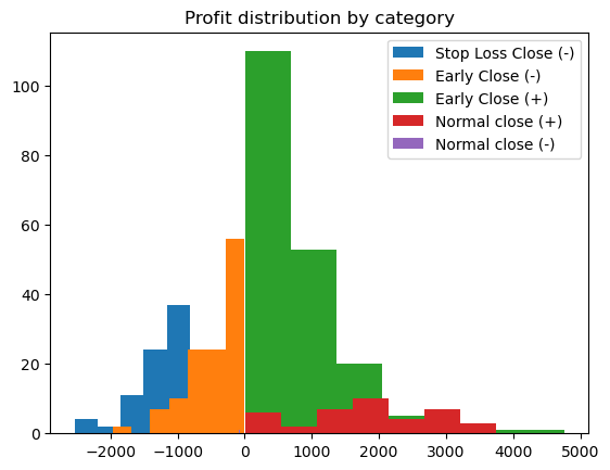 |
 |
| Close after one month | 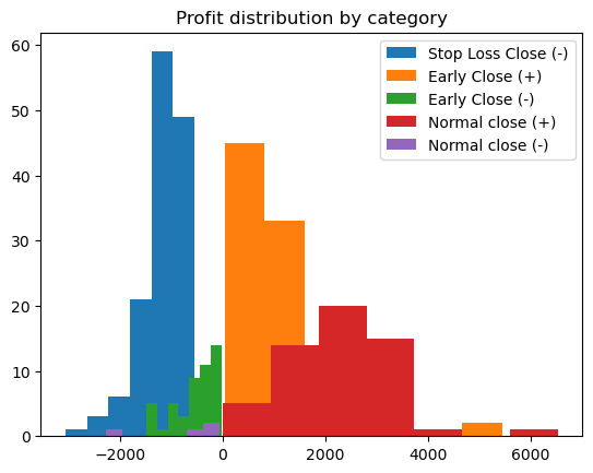 |
 |
| Close after six months | 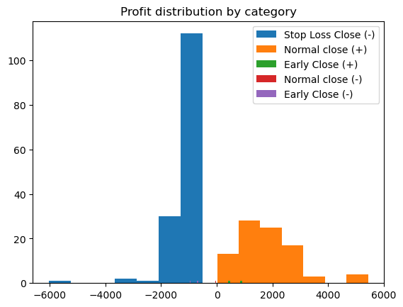 |
 |
| Close after one year | 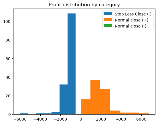 |
 |
Pair-wise performance of every scenario
From the charts above, you can tell that the volume of the Stop Loss orders increases while the holding period increase. That somewhat corroborates the inference stated in the paper An Anatomy of Pairs Trading: The Role of Idiosyncratic News, Common Information and Liquidity that the profits of pair trading do decrease along with the longer holding period. In the meantime, the volume of the Normal Close and Early Close (+) orders remain fairly stable. The full distribution charts above show that the cointegrated pair has a lower probability to diverge once a specific amount of time has passed. The win rate statistics table provided below further back up our conclusion drawn.
| Early Close Win Rate | Total Win Rate | |
|---|---|---|
| price_10_dist | 60.83% | 50.43% |
| price_22_dist | 66.67% | 44.13% |
| price_132_dist | 50.00% | 38.31% |
| price_1264_dist | N/A | 38.02% |
| log_price_10_dist | 61.31% | 51.22% |
| log_price_22_dist | 73.63% | 54.95% |
| log_price_132_dist | 75.00% | 40.56% |
| log_price_1264_dist | 100.00% | 35.33% |
Pair-wise performance of every scenario II
Take away
In this post, I have shown you how to implement the cointegration pair trading in detail step-by-step. There are two potential defects in our trading strategy that we detected once we release the trading script to the live environment, and theoretical-based and trustworthy solutions have been applied to mitigate the consequences brought by these defects. Lastly, we use this complete backtest to confirm that the profitability of each trading pair does make a difference given using different holding periods to safeguard your strategy from being sabotaged by time volatility. Hope you enjoy reading this post, and let me know if you would like to know any parameter that might impact the performance of the cointegration pair trading strategy, let me know.