Cointegration is a statistical technique to find out whether a time series closely follows the movement of the other time series. Therefore, it becomes an important technique in the pair trading strategy for us to determine the right stock pair to trade with. In this post, we’re going to see why traders prefer using the cointegration test over the correlation test in pair trading, and whether the cointegration test results can boost our trading performance.
Become a Medium member to continue learning without limits. I’ll receive a small portion of your membership fee if you use the following link, at no extra cost to you.
If you enjoy reading this and my other articles, feel free to join Medium membership program to read more about Quantitative Trading Strategy.
Previous researches
- 【Pair Trading】Part 1. Introduction to pair trading strategy
- 【Pair Trading】Part 2. 5 in-depth analysis of distance approach in pair trading
- 【Pair Trading】Part 3. The strategy that helps minimize your portfolio risk
From the results of the previous research posts, I’ve found out that the pair trading strategies using the distance approach and Pearson correlation approach are not as satisfying as I expected. Even though we’re able to achieve the goal of making our strategy market neutral and reducing the max drawdown drastically, our Sharpe Ratio of each strategy variation is also reduced to a relatively low level compared to the benchmark buy-and-hold strategy.
Since the first method in these five pair trading strategies, let’s start putting efforts into the second method and see whether this test can generate more insights to evaluate and then determine whether this is a profitable pair trading strategy.
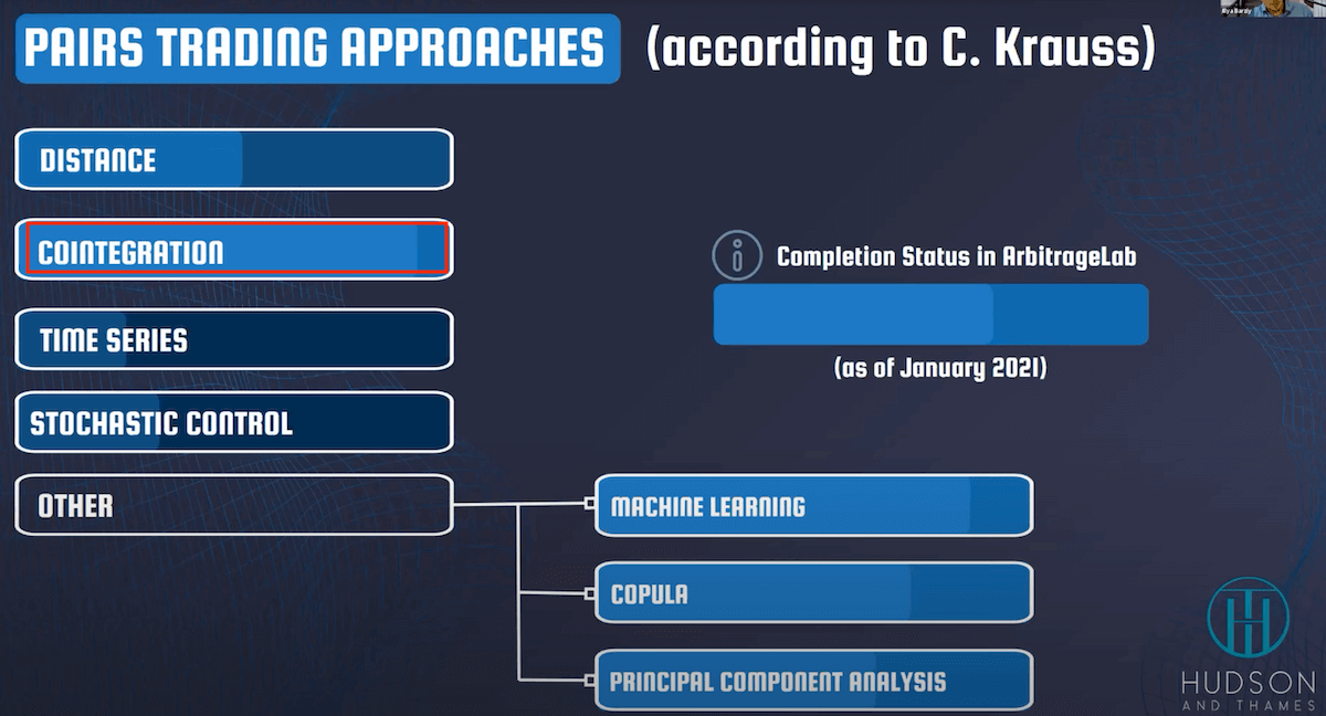
Extracted from Pairs Trading: The Distance Approach by Hudson & Thames
1. Lesson 101 of cointegration pair trading
1.1. What is Cointegration
Cointegration describes the relationship between time series in the long run. It is a milestone in the long history of studying multi-asset trading strategies. It first appeared in Granger’s seminal paper “Some properties of time series data and their use in econometric model specification” (Granger, 1981). When we put the term cointegration into the words of quantitative trading, cointegration helps us to find whether two stock prices have the spread (usually the difference of price or difference of log(price)) is stationary, indicating the mean and the variance of the spread stays the same in the observation period. This statistic feature meets the criteria of a mean-reversion strategy that involves two indifferent stocks.
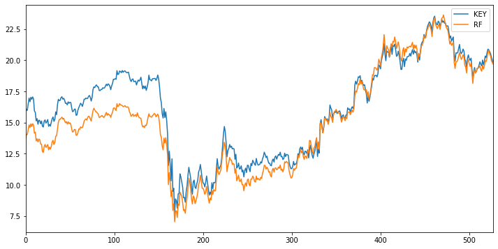
The price plot of KEY and RF
The price spread between KEY and RF will eventually go back to its mean value
But how do we examine whether the spread of two stock prices is stationary? Statistically speaking, a value in time series can be represented with the following equation:
By looking at the equation, we can tell that if the unit root $\alpha$ is greater than 1, the $Y_t$ is affected by the previous value $Y_{t-1}, Y_{t-2}, …$ in this time series and is no longer a random-distributed time series. Therefore, our goal is to see whether $\alpha$ exists, the smaller the better. If $\alpha$ doesn’t exist in this equation, then we can say that this time series is stationary as $Y_t$ is simply an add-up of $constant$ and a randomly-distributed $\epsilon$. Here’s where the Augmented Dickey-Fuller test (ADF test) comes into play. We use the ADF test to examine whether the unit root exists or not.
There are a lot of materials here for you if you would like to know more about what cointegration is about:
1.2. Misconception about the relationship between correlation and cointegration
One might say that, doesn’t the correlation test describe the same statistical feature as the cointegration test which both methods are trying to see whether two time series are moving towards the same direction in the same observation period?
Correlation is meant to examine and measure the linear relationship between two time series. The positive correlation (correlation > 0) means these two variables move in the same direction (up or down) over time, whereas the negative correlation (correlation < 0) means they move in different directions. On the other hand, the cointegration test doesn’t care how these two variables move together. Instead, it measures whether the difference between two variables remains constant over time. Therefore, high cointegration doesn’t necessarily exist if two time series are highly correlated.
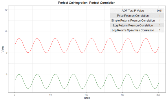
Time series that illustrates perfect correlation and cointegration - Rbloggers by cfsmith
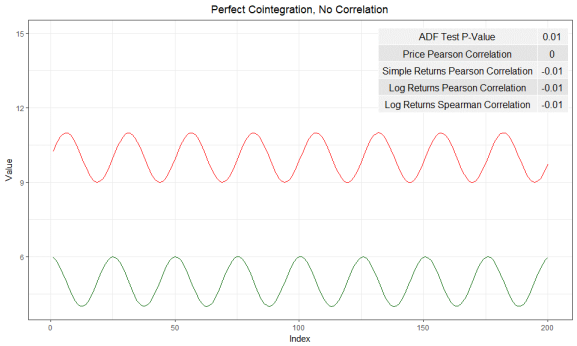
Time series that has perfect cointegration, but zero correlation - Rbloggers by cfsmith
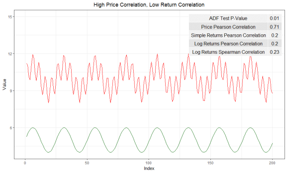
Time series has the same perfect cointegration, but has a relatively low correlation - Rbloggers by cfsmith
Reference:
1.3. The methodology
In this post, I choose to use Engle-Granger 2-step approach as it is the most commonly seen cointegration test process for pair trading. As the name tells, there are two steps to go through in order to find out whether the pair of stocks is suitable for this strategy:
First step
First of all, we use OLS as the regression method to get the residuals of the equation. The regression formula should look like this given both $x$ and $y$ are time series that we have:
By doing this, we can get the parameters $\beta$ and $constant$. Then we are going to calculate the residuals by using the following equation:
Now we save the residuals as the input of the second step.
Second step
The second step is much more straightforward. We use the Augmented Dickey-Fuller test to see whether the unit root exists in the residuals. If the hypothesis of having a unit root can be rejected by applying the Augmented Dickey-Fuller test, then we can say that the residuals are stationary and the time series $x$ and $y$ are cointegrated. Therefore, we can say this pair $\text{x-y}$ would be our trading target.
In python, it’s going to be as easy as:1
2
3from statsmodels.tsa.stattools import adfuller
adf_value, p_value= adfuller(TIME_SERIES_X, autolag = 'BIC')
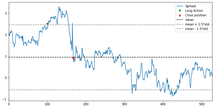
1.4. Trading rules
Theoretically speaking, the OLS-generated residuals should conform to the random distribution. That is to say, the cointegration pair trading strategy essentially is a mean-reverting, market-neutral, long-short strategy as the other pair trading strategy. The only difference is what would be the indicator to monitor and observe. In this case, we use the residual $\epsilon$ to generate the trading signals to either enter or exit a trade. Below is the most common trading rules performed in most of the research papers:
- Variables required
- Residuals ($\epsilon$) generated from the OLS regression: $\epsilon = y - \beta * x - constant$
- Mean of the residuals ($\mu$) as the benchmark line in our residual observation
- Standard deviation of the residuals ($\sigma$) to calculate the trigger line in our residual observation
- Threshold is a fixed value that uses together with the standard deviation of the residuals to calculate the trigger line. In this research, we set it to 2.32 for calculating the upper bound and -2.32 for calculating the lower bound. (2.32 is usually used as it includes 99% inside the normal distribution)
- Trading rules
- Generating enter trading signals
- Open a long position if the current spread is smaller than the mean of the spread $\mu - threshold * \sigma$
- Close a long position if the current spread is bigger than the mean of the spread $\mu$
- Open a short position if the current spread is bigger than the mean of the spread $\mu + threshold * \sigma$
- Close a short position if the current spread is smaller than the mean of the spread $\mu$
- Exit trading signals
- residual cross the mean of the residuals
- Repeated trading signals
- Only process the first signal if there are two consecutive enter/exit signals
- Generating enter trading signals
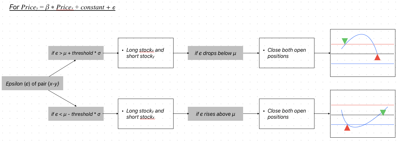
Pair trading rules flow chart
To make our trading rules more intuitively easier to understand, let’s have a look at the below chart:
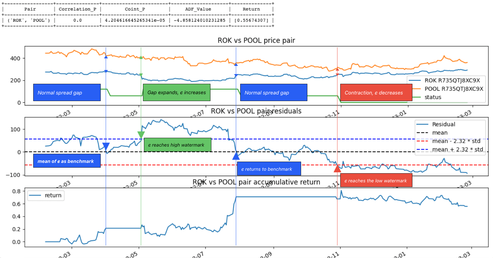
Top: Pair pricing movements; Middle: Residual movement; Bottom: Accumulative return (%)
2. Research plan
2.1. Goal of this research
Before starting to backtest the strategy performance, there are a few things that I would like to understand beforehand. Therefore, I set up three sets of scenarios to validate the answers to the below questions:
- When doing regression, whether stock price or log(price) will give us an edge?
- Do we need to filter out those pairs whose correlation is low before the cointegration test?
- Does the scenario using the pair in the same industries will have a lot of difference in performance compared to the scenario using the pair in different industries?
I believe having a clear view of the above questions will help conduct backtest in the later stage. So let’s get started!
2.2. Platform
2.3. Fetching data needed
In this research, we use 24 months of data as training data and feed them into the ADF test and OLS regression to get the results forming the pairs we need for the following steps. Once the pairs have formed, we’re going to use another 12 months of data as testing data to see whether the pairs with high cointegration intention would have the character of mean-reversion.
1 | formation_period = 22 * 24 |
2.4. Universe and implementation
I’m using the component stocks from S&P500 at one point as the base universe to start with. After downloading all the historic pricing data, I fed the necessary data into the following class to build the screening criteria:1
2
3
4
5
6
7
8
9
10
11
12
13
14
15
16
17
18
19
20
21
22
23
24
25
26
27
28
29class Pair:
def __init__(self, symbol_a:str, symbol_b:str, rtn_a, rtn_b):
self.symbol_a = symbol_a
self.symbol_b = symbol_b
self.rtn_a = np.array(rtn_a)
self.rtn_b = np.array(rtn_b)
self.corr, self.corr_p = self.correlation()
self.ols_hedge_ratio, self.ols_intercept, self.coint_value, self.coint_stationary_p, self.ols_res = self.cointeration_test()
def correlation(self):
# calculate the sum of squared deviations between two normalized price series
corr, p = pearsonr(self.rtn_a, self.rtn_b)
return corr, p
def cointeration_test(self):
x = self.rtn_a
y = self.rtn_b
x = sm.add_constant(x)
model = sm.OLS(y, x).fit()
intercept = model.params[0]
beta = model.params[1]
adf_result = adfuller(model.resid, autolag = 'BIC')
adf_value = adf_result[0]
stationary_p_value = adf_result[1]
return beta, intercept, adf_value, stationary_p_value, model.resid
Then here’s how I feed the data into this defined class:1
2
3
4
5
6
7
8
9
10
11
12
13
14
15
16
17
18
19
20
21
22# This is for storing the final results
pair_corrs = {}
for stock_pair in tqdm.tqdm(symbol_pairs):
if str(stock_pair[0]) not in history_price.columns:
# print(f'{str(stock_pair[0])} not in the history_price table')
continue
if str(stock_pair[1]) not in history_price.columns:
# print(f'{str(stock_pair[1])} not in the history_price table')
continue
if SPREAD_MODE == LOG_PRICE_MODE:
tmp = np.log(training_data.loc[:, [str(stock_pair[0]), str(stock_pair[1])]].dropna())
elif SPREAD_MODE == PRICE_MODE:
tmp = training_data.loc[:, [str(stock_pair[0]), str(stock_pair[1])]].dropna()
pair_corrs[(str(stock_pair[0]), str(stock_pair[1]))] = Pair(
str(stock_pair[0]),
str(stock_pair[1]),
tmp.loc[:, str(stock_pair[0])],
tmp.loc[:, str(stock_pair[1])]
)
Once the above actions have been accomplished, I’m choosing only the pairs whose ADF test p-value is smaller than 0.05 to be our candidates for pair trading:1
final_pairs = {key:value for key, value in pair_corrs.items() if value.coint_stationary_p <= 0.05}
Lastly, let’s sort the pairs first by their correlation value and then by their cointegration p-value. By doing this, it’ll be easier for us to conduct our stratified analysis based on their level of cointegration.
1 | final_pairs = {k:v for k,v in sorted( |
2.5. Results
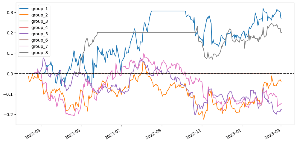
To better visualize our results, I’m going to compare different scenarios simply based on the visualized diagram using stratified analysis and accumulative return diagram from the top 20 stock pairs that have the lowest ADF test p-value. In the stratified analysis, I expect to see if the accumulative returns of each group are parted from each other and are ranked from group 1 (the lowest cointegration p-value) to group 8 (the highest cointegration p-value). As for the accumulative return diagram from the top 20 stock pairs, undoubtedly seeing a soaring return without a huge max drawdown would be the optimal result.
2.5.1. Using simply stock price v.s. log(stock price)
In the blog post Cointegration Trading with Log Prices vs. Prices by Dr. Ernest P. Chen, the difference between using price and using log price has been stated clearly:
For most cointegrating pairs that I have studied, both the price spreads and the log price spreads are stationary, so it doesn’t matter which one we use for our trading strategy. However, for an unusual pair where its log price spread cointegrates but price spread does not (Hat tip: Adam G. for drawing my attention to one such example), the implication is quite significant.
- Ernest P. Chen
Therefore, it would be interesting to see how this impact the entire strategy return.
| Price | log(Price) | |
|---|---|---|
| Industry pairs without correlation filter | 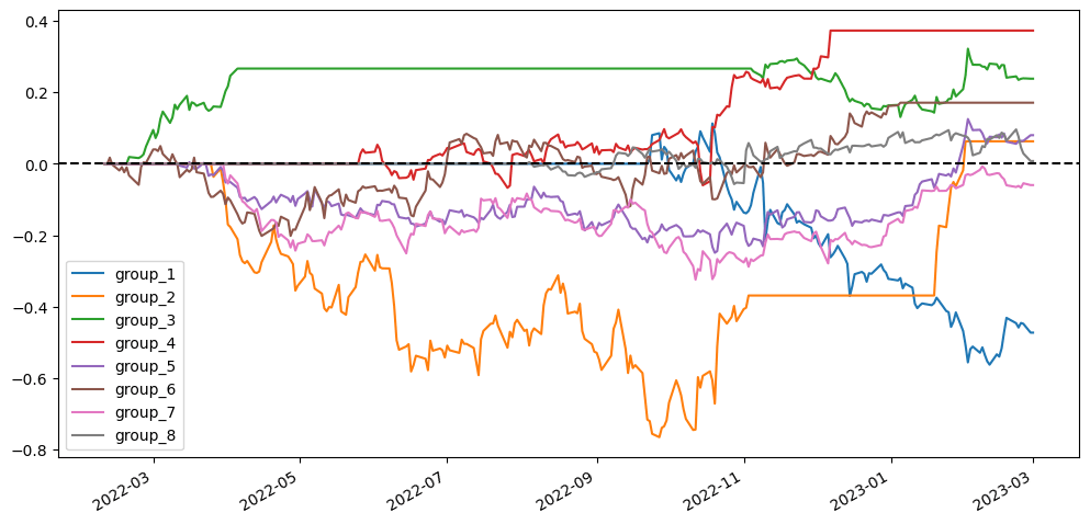 |
 |
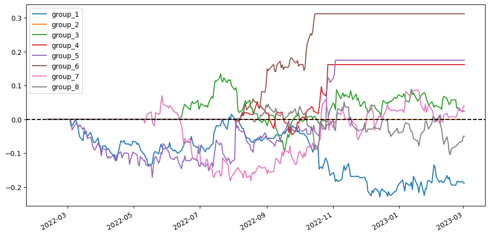
| Non-industry pairs without correlation filter | 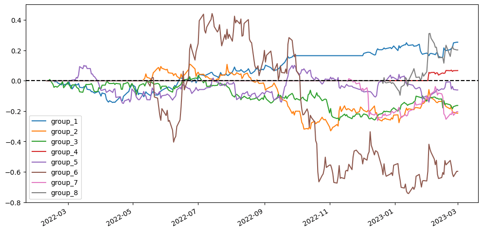 |
 |
| Industry pairs with correlation filter | 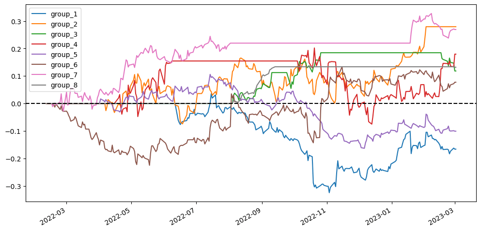 |
 |
| Non-industry pairs with correlation filter | 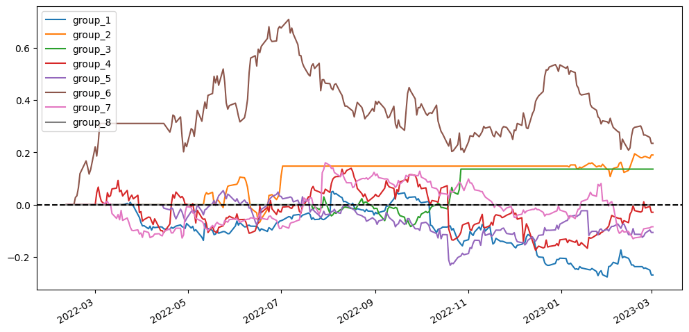 |
 |
The scenarios using log(price) don’t seem to have distinct differences from the scenarios using price. So we can’t say for sure that whether using price or log(price) is superior.
2.5.2. Filter by correlation + cointegration v.s. filter by cointegration
In this second research, I would like to know whether a high correlation has any positive impact on this trading strategy. The way I run this research is that, in addition to the already-have cointegration p-value filter, I add another filter to eliminate the pairs where the correlation value is under 0.9 and the p-value is greater than 0.05. Then, we do everything the same as the previous research.
| with correlation filter | without correlation filter | |
|---|---|---|
| Industry pairs with price | |
|
| Non-industry pairs with log(price) | |
|
| Industry pairs with log(price) | |
|
| Non-industry pairs with price | |
|
Somehow it seems that the scenarios without the correlation filter are always better performed than the corresponding scenarios with the correlation filter. This might give us a clue that maybe the correlation filter is not needed.
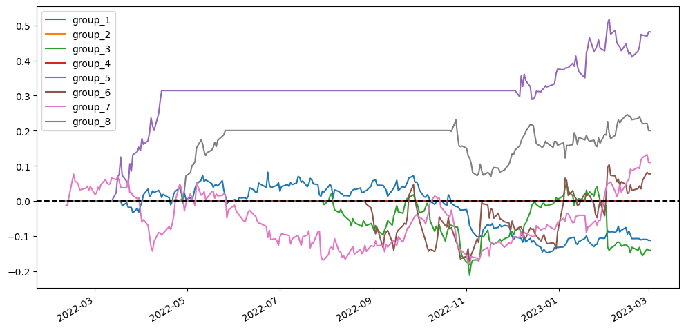
2.5.3. Construct pairs within the same industries or across different industries
As we all know that the stock prices of companies in the same industry tend to be impacted simultaneously by the economic or industrial incidence, which we can deduce that companies in the same industry could have higher cointegration relationships than companies in different industries. Is this true? And how will it impact our pair trading strategy? I construct the trading pairs in two different ways: 1. we make all possible combinations using the native python function itertools.combinations(). 2. we only make possible combinations when two companies are in the same industry.
1 | pairs = [] |
| Pairing within the same industry | Pairing across different industry | |
|---|---|---|
| Price with correlation filter | |
|
| Price without correlation filter | |
|
| log(price) with correlation filter | |
|
| log(price) without correlation filter | |
|
Same to previous research results, the first group returns in scenarios that form pairs across different industries seem always better than the ones in scenarios pairing within the same industry. That might tell us the cointegration relationship also exists across industries.
3. Conclusion
From the research above, we have gained some insights regarding how each factor impacts the performance of the pair trading strategy. But, are we able to answer the three questions we mentioned above with 100% confidence? No. There are more details that we need to take into account when conducting the backtest, such as:
- Update the universe periodically by recalculating the cointegration p-value of all the pairs.
- Use a smaller threshold to generate trading signals as the smaller entry point and exit will get a shorter holding period and more round trip trades and generally higher profits.
- Use z-score method to smooth the $\epsilon$ that we’re tracking.
- Close early if the trades were opened for too long.
- Add a stop-loss threshold to prevent losing more if the $\epsilon$ goes way beyond the threshold.
- …
A lot of techniques can be experimented with and tested during backtesting. In the next episode, I’m going to work on the backtest and see whether there’s a possibility that we can find a profitable cointegration trading strategy.
Cheers!