The Triple barrier method and meta-labeling technique were together introduced in the book Advances in Financial Machine Learning by Marcos Lopez De Prado. It seems that the combination of these two tools makes a great pair to either stabilize or further increase your portfolio growth. In this post, I’m going to quote my old research result (here) from last time as the fundamental strategy benchmark, and apply these two techniques to see what beneficial impact we could bring to this strategy.

Previous researches

Motivation

After researching the combination of several technical indicators as buy-in signals, I feel the research framework is missing a robust method to mitigate the subjective impact of the technical indicators. Theoretically speaking, stock prices and other statistics represent the current market overview. Using this information to predict future stock price movements would be irrational. However, standing from the behavioral finance point of view, the historic stock prices and statistics could be used to summarize the standard behavior of general investors’ actions when certain critical points were reached. That’s where the momentum trading strategy begins to thrive. Traders/Investors combine several effective indicators and define the fixed or dynamic threshold to find the group of stocks that possess the momentum (uptrend or downtrend) in them. Then the problem comes back to, how do we define the threshold in a more objective method.

In the book Advances in Financial Machine Learning by Marcos Lopez De Prado, the Triple barrier method (Chapter 3.4) and the meta-labeling technique (Chapter 3.6) were introduced with his quote “In that case, meta-labeling will help us figure out when we should pursue or dismiss a discretionary PM’s call” (Page 54). These two tools could be adopted and leverage the power of machine learning to mitigate the subjectiveness in the technical-indicator-oriented momentum strategy.

As usual, I’m not going to introduce these two ideas from ground zero. The article What is Triple Barrier Method(TBM) and Meta-labeling breaks down the definitions of these two terms and attaches the code snippet for easier comprehension. See below for you to understand what they are.

The definition of the Triple Barrier Method (TBM)

TBM adopts two horizontal lines and one vertical line to form a box, which is used for deciding the next move depending on the relative position of the stock price inside the box. There are three potential scenarios would be produced:

If the upper barrier (profit-take) is hit first. Label “buy” or “1”.
If the lower barrier (stop-loss) is hit first. Label “sell” or “-1”.
If the vertical barrier (expiration) is hit first. Label = “return in this period” or “0”.

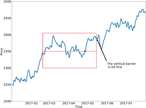
Triple Barrier Method Scenario 3 - hitting the vertical barrier

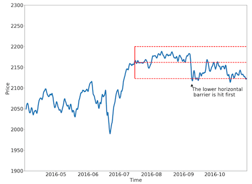
Triple Barrier Method Scenario 1 - hitting the horizontal barrier

The definition of the meta-Labeling

The meta-Labeling sounds like simply an extra label, but it is actually a term that indicates a series of actions for getting the final prediction at the end. This Youtube video by Hudson & Thames successfully summarizes the core idea of Meta-labeling:

Meta-labeling is a machine learning (ML) layer that sits on top of any base primary strategy to help size positions, filter out false-positive signals, and improve metrics such as the Sharpe ratio and maximum drawdown.

The steps to implement the meta-labeling can be summarized in the followings:

Build the primary fundamental model and get the fundamental prediction.
Use a fixed value to filter the prediction.
Combine the prediction into your x_train as your new training data.
Combine the prediction into your y_train to form the new y_train data.
Construct the secondary model, and use your new x_train and y_train to train your secondary model.
Feed your test_data into both your primary and secondary model, and produce the predictions respectively.
Combine the predictions of both the primary and secondary models in order to acquire your final prediction.

Meta-Labeling process

You might have questions right now as you just read my previous post and ask “weren’t the Meta-labeling and the ensemble learning referring to the same thing?” The fundamental difference between these two is that ensemble learning (especially the stacking method) solely adds its prediction into the original training set as a new feature. On the other hand, the meta-labeling not only adds its own prediction into the training set, but also modifies the y_label in the training set in accordance with the signal generation logic from the primary model. By having general ideas of what these two are, we can start strategizing how to achieve our goal from zero to one.

Train of thought - from zero to one

To accomplish this backtest, I’ve summarized five steps below to give you a big picture of what we’re going to do:

Construct our primary model and generate meta label using our primary model
Use our modified Triple-Barrier Method to generate training data for training our secondary model
Construct the secondary machine learning model
Train the secondary model
Execute and place orders with the combined signals.

1. Construct our primary model

First of all, we use the strategy left from here and use the buy/sell signals generated from it as the Meta-label. We used MACD, Awesome Oscillator, and RSI indicator to generate our trading (buy/sell) signals. Other than this, we also prepare the following factors for later use:

FEATURES = [
  '_1d_rtn', '_3d_rtn', '_5d_rtn', '_10d_rtn', '_20d_rtn', '_60d_rtn',
  '_1d_volume_change', '_3d_volume_change', '_5d_volume_change', '_10d_volume_change', '_20d_volume_change', '_60d_volume_change',
  '_macd', '_macd_histo', '_macd_change_3', '_macd_change_5', '_macd_change_10', '_macd_change_15',
  '_macd_signal_change_3', '_macd_signal_change_5', '_macd_signal_change_10', '_macd_signal_change_15',
  '_macd_histo_change_3', '_macd_histo_change_5', '_macd_histo_change_10', '_macd_histo_change_15',
  '_rsi', '_rsi_change_3', '_rsi_change_5', '_rsi_change_10', '_rsi_change_15', '_awesome_oscillator',
]

Factors to be used in the second machine learning model

2. Modified Triple-Barrier Method

In the original Triple-Barrier Method, the difference between the first and second vertical barriers indicates the expiration time that is a fixed number. However, the sell signal generated from our primary model could happen before reaching the expiration time. Secondly, we’re not able to predict the exact time between the buy signal and sell signal as each stock would have its own cycle and price movement velocity. Therefore, we need to slightly twist the definition of expiration time in Triple-Barrier Method by defining different expiration times for each stock base on the time between the time of generating the buy signal and the time of generating the sell signal.

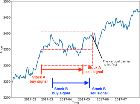
Modified Triple-Barrier Method using buy/sell signals to form a close period

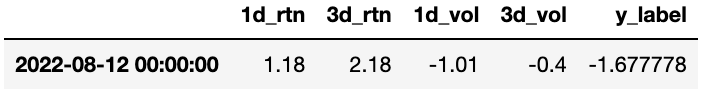
Since we have defined the expiration time, then we need to resample the original training data into a usable and meaningful format. For example, if we have a time series data that includes ‘price’, ‘1d_rtn’, ‘3d_rtn’, ‘1d_vol’, and ‘3d_vol’ as follows:

Example data - 1

Once we have the original data, now let’s generate the buy and sell signal with it and attach the signals generated to its own row. You can easily mark the row that has one buy signal and one sell signal.

Example data - 2

Lastly, just as we will do when resampling the data, we keep all the factors in the row that has buy signal equal to True. We calculate return gain/loss between the buy and sell signals. Then we remove the column ‘price’, ‘buy signal’, and ‘sell signal’. In the end, we will have our training data that is used for training our secondary model.

Example data - 3

3. Construct our secondary machine learning model

Here I use the basic neural network machine learning model to predict the winning stocks. There are two hidden layers in the model. Second, we use Leaky ReLU as the activation function of the hidden layers as I want the negative values to be able to update our model weights instead of doing nothing. I found this post very useful to understand the differences among various activation functions such as GELU, SELU, ELU, ReLU, and Leaky ReLU. Also, since it’s going to be a binary classification to predict whether the trades we made are profitable or not, we’re using binary_crossentropy as our loss function.

See below for the summary of my neural network setup:

self.model = tf.keras.Sequential()
self.model.add(tf.keras.layers.Dense(len(FEATURES), activation=tf.keras.layers.LeakyReLU(alpha=0.01), input_shape=(len(FEATURES), ), name="dense_1"))
self.model.add(tf.keras.layers.Dropout(0.1),)
self.model.add(tf.keras.layers.Dense(len(FEATURES), activation=tf.keras.layers.LeakyReLU(alpha=0.01), name="dense_2"))
self.model.add(tf.keras.layers.Dropout(0.1)),
self.model.add(tf.keras.layers.Dense(1, activation="sigmoid", name="predictions"))

# Compile model
self.model.compile(
    optimizer='Adam',
    loss='binary_crossentropy',
)

4. Training and predicting

Since having our training data and our secondary model ready in steps 2 and 3, we are now going to feed the data into our machine-learning model and start training. Before that, do remember that our data is raw and could have many outliers and missing data that could potentially contaminate the results of the prediction. Feature engineering is a must-take step. Here are a few things I did before throwing data into the black box:

def PrepareData(self, data):
  '''Prepares the data for a format friendly for our model'''
  target_column = 'rtn_bin'
  data = self.__LabelYData(data, '_y_trade_rtn', target_column)

  data_tmp = data.dropna()

  X_train = data_tmp.loc[:, FEATURES]
  y_train = (data_tmp.loc[:, target_column]).astype(int)

  X_train = self.__WinsorizeCustom(X_train, FEATURES)
  X_train = self.__LogCustom(X_train, LOGNORMAL_FEATURE)

  return X_train, y_train

def __LabelYData(self, df, source='_y_trade_rtn', rtn_bin='rtn_bin'):
  pass

def __WinsorizeCustom(self, df, cols: list):
  pass

def __LogCustom(self, df, cols: list):
  pass

4.1. Create y_label to train our model

We need our dependent variable, the so-called y label, to train our secondary machine learning model. There are various ways to achieve this. I pick the easiest method to create the y label by assigning True to the stock that its return is greater than 3.0% after we sell it. You can pick other methods and see which better suits your scenarios and models.

def __LabelYData(self, df, source='_y_trade_rtn', rtn_bin='rtn_bin'):
  df[rtn_bin] = np.nan

  df[rtn_bin] = df[source] > 0.03

  return df

4.2. Winsorize the outliers

Winsorization is the process of replacing the values of outliers with the less impactful smaller values. Here in order to reduce the impact of extreme values, we use the 5 percentile value to replace the extremely small value, and use the 95 percentile value to replace the extremely large value.

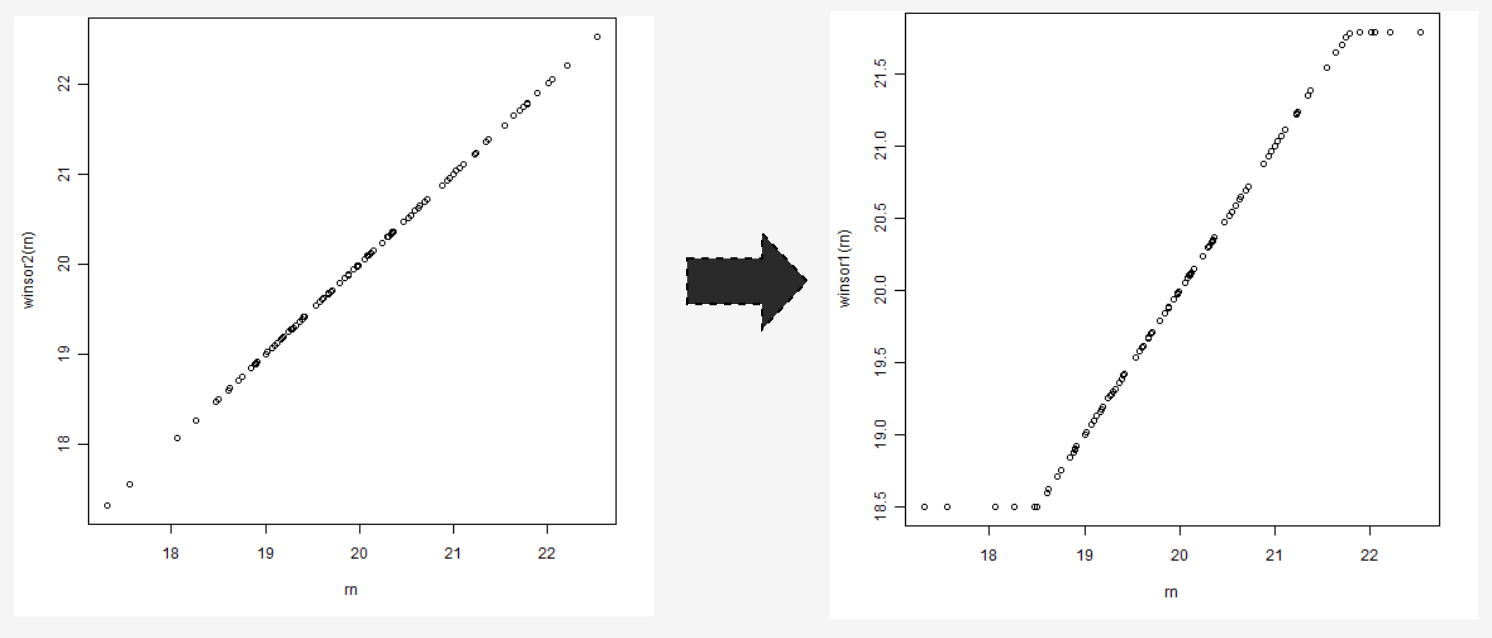
Winsorization

def __WinsorizeCustom(self, df, cols: list):
  for col in cols:
    quantiles = df.loc[:, col].quantile([0.05, 0.95])
    q_05 = quantiles.loc[0.05]
    q_95 = quantiles.loc[0.95]

    df.loc[:, col] = np.where(
      df.loc[:, col].values <= q_05,
      q_05,
      np.where(
        df.loc[:, col].values >= q_95,
        q_95,
        df.loc[:, col].values
      )
    )
  return df

4.3. Transform our data to the log-normal distribution

It’s a well-known fact in financial machine learning, that having our data normally distributed is the prerequisite of an effective machine learning model. After plotting each of the factors in the histogram, you can easily tell which feature is skewed, then you apply log transform to make it less skewed. One thing that is worth bringing up again, is that some features could contain a 0 value. Since log 0 doesn’t exist and will return NaN, causing model training to fail, make sure you add 1 before you log transform the feature values.

Transform the right-skewed distribution to normal distribution

def __LogCustom(self, df, cols: list):
  for col in cols:
    df.loc[:, col] = np.log(df.loc[:, col] + 1)
  return df

4.4. Drop the null data

Don’t forget to trim the null data. Otherwise, your model is going to fail while training and predicting.

5. Execute and place orders with the combined signal

Lastly, to summarize, our trading strategy would be that when we receive the signal from the primary model, we send the data on the day as the testing data for predicting with the secondary model. Once the secondary model confirms the signal with the prediction higher than 0.5 possibility to be a winning trade, then we place the buy order. As for selling the stock, we don’t need confirmation from the secondary model. As long as the primary model confirms and generates the sell signal, we sell the related holding stock.

Backtesting and result

Ok. Let’s see what the backtesting results look like following the strategy that we describe above. I will start by describing the backtesting scenarios that we’re going to perform, and then demonstrate the results.

Platform

QuantConnect

Universe

Sort stocks by PERatio, EPS, ROE, NetIncome and take top 60%
Sort stocks by PBRatio, from high to low
Focus on technology industry
Using QQQ as the portfolio benchmark

Rebalancing Strategy

Recalculate our universe and indicators to search for the buy and sell signals every day.
We keep 10 stocks that have buy-in signals and with the highest PBRatio.
We assign weight to each position evenly.
We don’t adjust the weight of each stock until we close these positions.
The secondary model will be re-trained monthly, weekly, and daily.

Backtest time frame

Backtest Date: 2018, 12 ,29 ~ 2022, 09, 24

Execution and backtest

Scenarios

There are two strategies in our arsenal and I’m going to try them out. I’m also going to take the frequency of updating our model into consideration by retraining the model with the up-to-date data every month, week, and day. Therefore, there are going to be six scenarios and two basic scenarios as our benchmark strategy in our backtests.

1. MACD strategy benchmark
2. MACD strategy + Update monthly
3. MACD strategy + Update weekly
4. MACD strategy + Update daily
5. MACD+RSI strategy benchmark
6. MACD+RSI strategy + Update monthly
7. MACD+RSI strategy + Update weekly
8. MACD+RSI strategy + Update daily

Backtesting results

Strategy	Total Trades	PSR	Unrealized	Fee	Return	Sharpe	MDD	Win rate	Alpha	Beta	Annual variance
MACD Benchmark	838	23.299%	-$29,616.40	-$4,091.44	146.89%	0.787	42.300%	67%	0.119	1.053	0.087
MACD Monthly	928	14.622%	-$30,950.28	-$4,372.03	79.55%	0.587	44.700%	66%	0.038	1.067	0.068
MACD Weekly	834	21.410%	$-25,909.75	-$3,761.04	150.54%	0.773	41.200%	68%	0.125	1.074	0.096
MACD Daily	832	28.575%	$-36,755.89	-$4,177.46	182.07%	0.88	42.500%	68%	0.154	1.02	0.09
MACD+RSI Benchmark	1270	18.732%	$-14,361.51	-$6,592.32	96.85%	0.665	43.200%	58%	0.063	1.014	0.067
MACD+RSI Monthly	941	14.348%	$-7,308.52	-$4,382.58	72.05%	0.575	46.900%	56%	0.036	0.946	0.057
MACD+RSI Weekly	829	1.204%	$-436.44	-$3,535.95	-7.91%	0.03	56.000%	54%	-0.077	0.771	0.042
MACD+RSI Daily	898	19.534%	$-7,414.81	-$4,494.80	92.44%	0.679	43.000%	56%	0.065	0.89	0.056

Beyond and next

The purpose of Meta-labeling is not just for correcting the false-positive prediction, but also for raising the F1 score of the model. By adding another machine learning layer beyond the primary non-machine learning model, Meta-labeling enables the capability of processing quantitative fundamental data, technical indicators, and even arbitrary data in a more systematic way. This combines human intuition/experience and the power of machines, enhancing the interpretability and robustness of the model.

Even though the backtesting results failed to demonstrate the overwhelming power of the meta-labeling, there are still a few other thoughts and ideas to extend our backtesting and to further optimize our Meta-labeling trading algorithm:

Add company-wise fundamental data into our training data to let our secondary machine learning model know more about the conditions and hence make better decisions.
In our backtest scenario, we round the prediction result and make it either True or False. That means the threshold is 0.5 that prediction lower than 0.5 would be deemed as a potentially losing trade, and the number above 0.5 would have a higher chance to become a winning trade. One thing we can do is to raise the threshold bar from 0.5 to a higher number to make sure you have an even higher chance to win in this trade. But keep this in mind, it’s going to be a trade-off between the number of trades and you could let the winning opportunities slip through your fingers.
Find a better method to label your y-label in order to distinguish the stocks that are going to soar or decline. You could either raise the original 3.0% to a bigger number or mark the top 20% winning stocks so that our y-label will not be restricted to only the winning stocks during the bear market.

Reference

The book Advances in Financial Machine Learning by Marcos Lopes De Prado
Labeling financial data for Machine Learning by Amir Masoud Sefidian
Meta-Labeling: Theory and Framework - Youtube video by Hudson & Thames

If you enjoy reading this, feel free to join Medium membership program to read more about Quantitative Trading Strategy.

Michael's blog

【Momentum Trading】Use machine learning to boost your day trading skill - meta-labeling