
When it comes to using machine learning algorithm to pick the stocks that are most likely to produce a good return, it is similar to seeking the opinion of an investment consultant. However, it can be unsettling to make your investment decision after listening to just one consultant. Now is the moment to get second opinions and hire more investment advisors to make sure the investment concept is reliable, doable, and profitable.
The same principle that you consult other machine learning algorithms to confirm the predictions made by these models are applied in ensemble learning. When you have collected all of the final data from these models, you may take your time relaxing in your nice chair like a big boss, analyzing the results, and making your important and sacred decision.
Motivation
In the previous articles 1 2 3 4 and 5, we have built the machine learning script to predict the winners in the stock market using only the XGBoost model. Nevertheless, there are many algorithms out there for us to try and evaluate. So the most important question for us becomes much more complex. We need to build multiple machine learning models, use GridSearch to find the best hyperparameters, train/fit many different machine learning models, evaluate each model with the same metrics, pick the best-performing model for us to use, and …….
How are we going to do this?
Ensemble learning
Ensemble learning is a method to combine the predictions from different machine learning models. We gave these machine learning models the name weak learners, as compared to our finalize machine learning model, these weak learners contribute only a part of their efforts to produce the final predictions. By saying that, the ensemble learning model is a more powerful predictor by using a strong learner to assemble the results from many weak learners, so that our final predictor is able to waive the variances from some of the machine learning models and also prevent the overfitting of a singular model. Below is the list of the ensemble learning techniques:
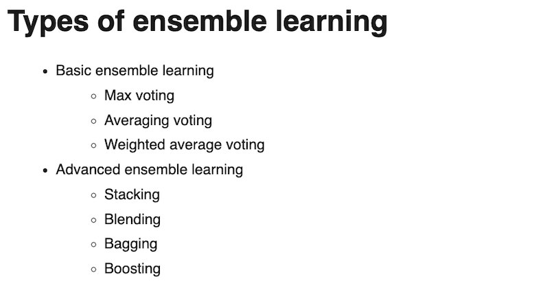
Different types of ensemble learning techniques
Pause!! Let’s narrow it down
Among these ensemble learning techniques, Bagging and Boosting are the most commonly known techniques. They are even used in the modern machine learning algorithm such as the Adaboost model or the XGBoost model that we used in our previous articles. However, to cover all these techniques would probably bore you to death. Therefore, we’re going to introduce two techniques in this article, Average Voting and Stacking. Also, as explaining the basic theory is not my strength, I’ll put less effort into explaining and more effort into describing the details of the backtests and coding details.
Average Voting
As the name implies, average voting is to average the predicted scores/probabilities from your weak learners and output the final scores/probabilities. For example, you have three weak learners classifier models trained and produced the final predicted probabilities of getting the positive return tomorrow.
| Classifier Model | Stock 1 | Stock 2 | Stock 3 |
|---|---|---|---|
| A | 0.9 | 0.9 | 0.7 |
| B | 0.7 | 0.3 | 0.7 |
| C | 0.6 | 0.7 | 0.7 |
| Averaged possibility | 0.73 | 0.63 | 0.7 |
Possibilities of getting the positive return tomorrow (Soft voting)
If we look at models A, B, and C respectively, we probably end up buying Stock 2 as it has a relatively high probability to receive a positive return from models A and C. After employing the average voting technique, the probability of Stock 2 now drops to 66% and Stock 1 probability would top Stock 2, indicating that Stock 1 would actually have a higher probability to receive a positive return than the other two stocks. This is so-called Soft Voting.
There is also Hard Voting, which takes binary inputs, True or False, into account instead of the probabilities. Taking the same example as above, we add one more condition that the output would be 1 (True) only when the possibility is over 0.7. The final result would be quite different.
| Classifier Model | Stock 1 | Stock 2 | Stock 3 |
|---|---|---|---|
| A | 0.9 (1) | 0.9 (1) | 0.7 (1) |
| B | 0.7 (1) | 0.3 (0) | 0.7 (1) |
| C | 0.6 (0) | 0.7 (1) | 0.7 (1) |
| Voter | 2 Positives & 1 Negative | 2 Positives & 1 Negative | 3 Positives |
Possibilities of getting the positive return tomorrow (Hard voting)
By looking at the total number of the voters who vote positive, the final winner would be Stock 3 as it has 3 people who think it’s going to receive a positive return tomorrow. Therefore the Hard Voting would recommend Stock 3, yet the Soft Voting would recommend Stock 2. The concept is quite straightforward, but this technique does help the model to mitigate the impact of the high variance of one single model.
Stacking
Other than average voting, Stacking processes the predictions from the weak learners in a more advanced way. Stacking treats the outputs of its weak learners as features and stacks them together into secondary training data. The secondary training data will be used as the inputs for the final estimator (a.k.a. meta-model), and then computes the final prediction.
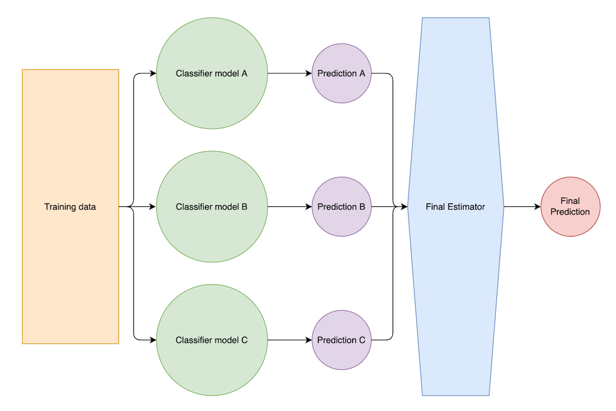
Stacking technique illustration
As illustrated above, classification models A, B, and C use the same training data to train the model and then produce predictions A, predictions B, and predictions C. The final estimator treats these predictions as new features to compute the final prediction.
Walk through the strategies
We now have the general idea of these two ensemble learning techniques, let’s move on to the backtest so that we can understand the power of ensemble learning. In this series of backtests, we are going to use the same dataset to train 1. XGBoost, 2. LogisticRegression, 3. SVM, and 4. Deep Learning with 2 layers of hidden layers. After conducting the backtests using these models respectively, we will combine these models together and apply Average Voting and Stacking techniques respectively to see whether the performances are improved or not.
Universe and training data
I’m still using ZZ500 as our universe and the same set of features as the training data. If you are interested in knowing how to define the universe and what features I’ve been using, you can check out my previous articles regarding machine learning and factor analysis.
Backtest timeframe
My backtest timeframe is from 2020-04 ~ 2022-07. For each month, I would need 60 months’ data as the training data to train the model. Therefore, it would require 27 (validation data) + 60 (training data) = 87 months = ~ 8 years of stock data.
Backtest scenarios
Here are the four models that I employed in this backtest. Again, I’m not the professor of the machine learning algorithm that can turn you into a machine learning expert with what I know. Instead, I’m going to put some quick descriptions and the materials that help me understand the basics of these ML models.
1. XGBoost
This is the decision-tree-base model that I’ve been using since the first article. The advantage of this algorithm is it’s extremely fast. This model took 1/5 of the time to train compared to other models. Below are the StatQuest videos that help me to understand what XGBoost is about:
- Gradient Boost Part 1 (of 4): Regression Main Ideas
- Gradient Boost Part 2 (of 4): Regression Details
- Gradient Boost Part 3 (of 4): Classification
- Gradient Boost Part 4 (of 4): Classification Details
- XGBoost Part 1 (of 4): Regression
- XGBoost Part 2 (of 4): Classification
- XGBoost Part 3 (of 4): Mathematical Details
- XGBoost Part 4 (of 4): Crazy Cool Optimizations
2. LogisticRegression
Logistic Regression is very much like the Linear regression that I talked about in 【Factor analysis】 Vol. 1. Introduction the idea of factor analysis. It uses various ordinal features to predict the probability of whether a thing will happen or not. To transform the probability into a Boolean value that stands for whether a certain incidence will happen or not, an activation function (such as Sigmoid or Softmax) will be applied. Here are the materials for you to know more about logistic regression:
- StatQuest: Logistic Regression
- Logistic Regression Details Pt1: Coefficients
- Logistic Regression Details Pt 2: Maximum Likelihood
- The SoftMax Derivative, Step-by-Step!!!
3. SVM
I have introduced the concept of SVM here. SVM is a variant of logistic regression. Instead of finding the exact line to separate all the 0’s and the 1’s, we include an extra hyperplane into the model. We hope that by adding this hyperplane, we will be able to clearly separate the data into different groups. The method for inserting this hyperplane is referred to as a ‘kernel.’
- Support Vector Machines Part 1 (of 3): Main Ideas!!!
- Support Vector Machines Part 2: The Polynomial Kernel (Part 2 of 3)
- Support Vector Machines Part 3: The Radial (RBF) Kernel (Part 3 of 3)
4. Neural Networks
The neural network is a type of deep learning algorithm. It uses numerous nodes to simulate the neuron in a neural system of a person, that each neuron makes individual solution and combine these solutions to make the final solution. Below are the related articles to talk about the NN model:
- TensorFlow Guide
- Tensors for Neural Networks, Clearly Explained!!!
- Neural Networks Pt. 1: Inside the Black Box
- Neural Networks Pt. 2: Backpropagation Main Ideas
- Neural Networks Pt. 3: ReLU In Action!!!
- Neural Networks Pt. 4: Multiple Inputs and Outputs
- Neural Networks Part 5: ArgMax and SoftMax
- Neural Networks Part 6: Cross Entropy
- Neural Networks Part 7: Cross Entropy Derivatives and Backpropagation
- Neural Networks Part 8: Image Classification with Convolutional Neural Networks (CNNs)
1 | def get_model(): |
My neural network model set up
5. Average Voting Algorithm
As previously explained, Average Voting essentially averages out the predicted scores/possibilities participated in machine learning models. Therefore, it’s relatively easy to implement the average voting model by putting your model into a list as an estimator parameter. The tricky part is, that the TensorFlow library that the neural network model uses is originally developed by Google, and the scikit-learn library that built the VotingClassifier is not. These two models are not naturally compatible and your neural network model can’t be tucked into the estimator parameter directly. Fortunately, TensorFlow also provides the function to wrap our NN model into a format that the scikit-learn library can understand. Hence, remember to wrap your NN model before you start building your Average Voting Algorithm.
1 | import TensorFlow as tf |
Use `tf.keras.wrapper.scikit_learn` to wrap our NN model
Once you have your models ready, you simply need to put them together into a list and add the wrapper to the VotingClassifier function. Here we use voting='soft' to smooth the variance of the model predictions.
1 | from sklearn.ensemble import VotingClassifier |
VotingClassifier basic instruction
6. Stacking
In our StackingClassifier, we use the XGBoost model, the Support Vector Machine model, and Neural Network models as our base estimators. As for the final estimator to produce the final prediction, we use the Logistic Regression model with the parameters needed. Once the model is instantiated, we can use this instance as the rest of scikit-learn model to fit and to predict. Make sure you include the hyperparameters before you build your base learner models.
1 | from sklearn.ensemble import StackingClassifier |
Basic set up of StackingClassifier
Backtest results
Backtest results summary
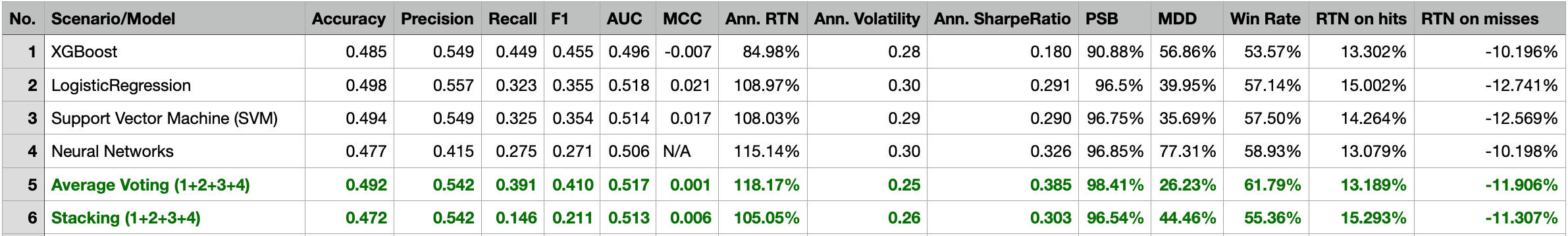
Backtest results summary
Even though the annual returns of both VotingClassifier and StackingClassifier are not higher than the other machine learning model, the Sharpe Ratio and the Maximum Drawdown are relatively lower. The win rate of the VotingClassifier scenario even increases to 61%, indicating our model is more powerful in its predictability to pick the stocks that are more possible to gain positive returns. To gain a more intuitive sense of how the ensemble learning method impacts our model, let’s look at the stratified and the return diagrams.
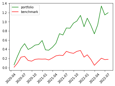
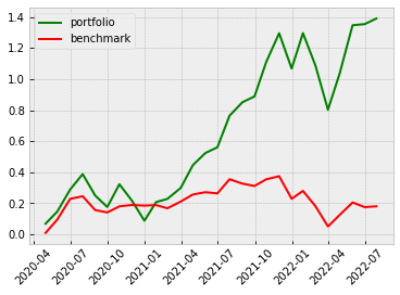
| Scenario | Stratified Diagram | Return Diagram |
|---|---|---|
| XGBoost | 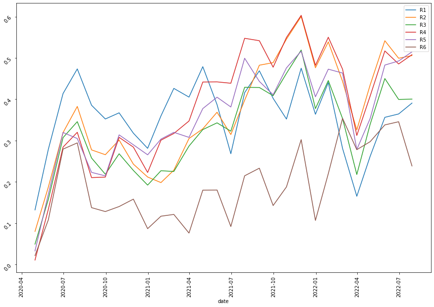 |
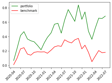 |
| Logistic Regression | 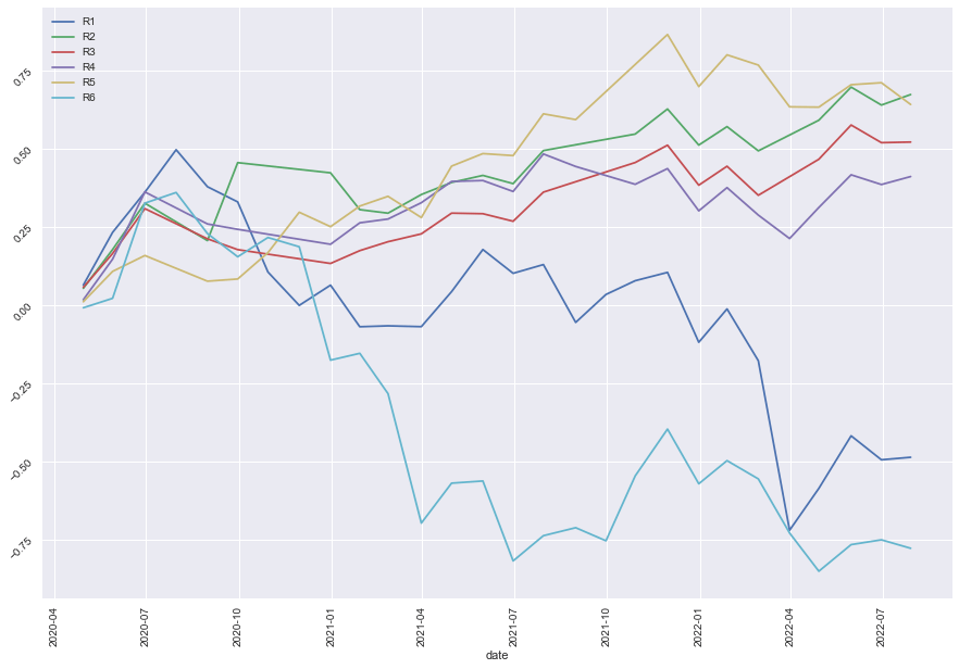 |
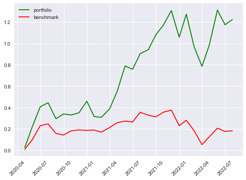 |
| SVM | 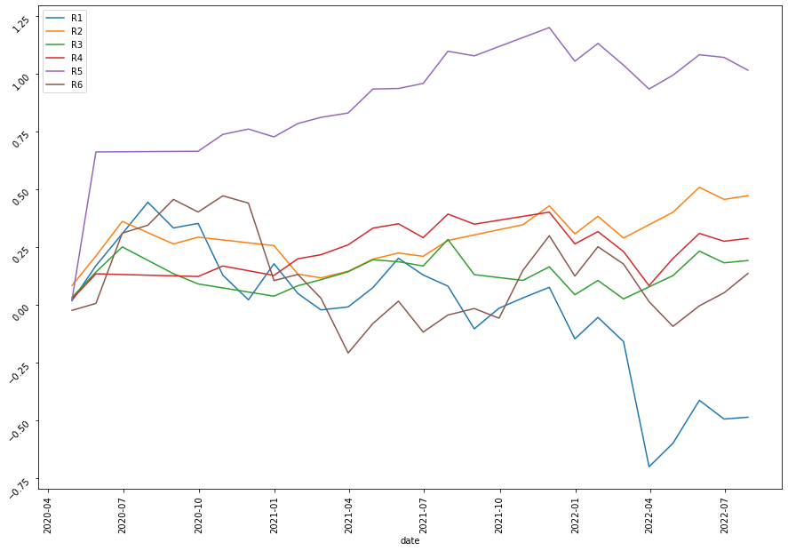 |
 |
| Neural Network | 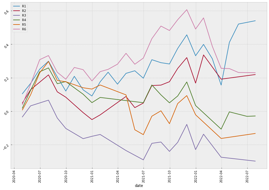 |
 |
| Average Voting | 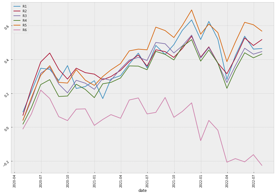 |
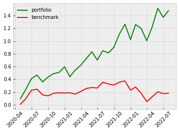 |
| Stacking | 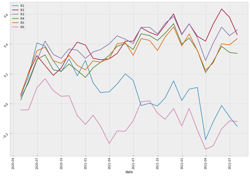 |
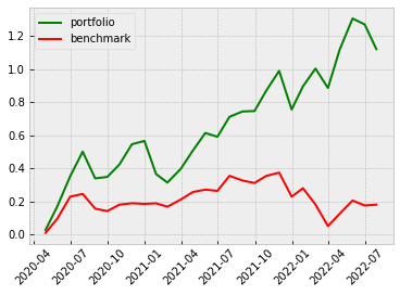 |
It’s quite clear that our ensemble learning methods (Average Voting and Stacking) less fluctuate than the rest of the models. By comparing the same bear market period from 2022-02~2022-04, our loss appears a lot less than the non-ensemble learning methods.
Conclusion
For the Average Voting ensemble learning method, it seems to produce a better result and improve the predictability of our model. However, there are a lot fewer places we can step in to better fine-tune the model. On the contrary, there is much more room for us to find out the best combination of the base estimators when we look at the Stacking ensemble learning method. Hence, one thing we can try is using the result from Average Voting as a benchmark and using Stacking as a tool to see whether we can build a much more powerful model to better predict the market.