
Photo by Brett Jordan on Unsplash
From the previous article, we’ve learned several indicators that we can calculate and use to evaluate the performances of your algorithm trading strategies. Given these indicators, we’re able to see how we can further polish our strategy and make it more seemingly profitable. Therefore, let’s work on our features to see how we can improve our machine learning trading strategy.
There are a few feature engineering techniques that we’re going to use in this series of backtests and it is beneficial to get a big picture of how to apply these techniques. I’m not going to go through these techniques in detail as there are too many capable persons who have done so. Therefore, I’ll be only focusing on backtesting the trading strategies using these techniques and how they can impact the performance of the strategy.
Also, I’m using the algorithm trading script that I built from my previous articles below. So we don’t need to build everything from the scratch.
Previous articles
- 【Machine Learning】 Part I - 10 minutes to learn what I know about machine learning in quantitative trading
- 【Machine Learning】 Part II - How to build a machine learning boilerplate?
- 【Machine Learning】 Part III - 5 myths about practicing quant trading with machine learning
- 【Machine Learning】 Part IV - How to analyze how good my machine learning strategy is?
Train of thought
There are three scenarios that we’re going to use as the benchmark performances:
- Using XGBoost as ML model and 30-month data as training data
- Using XGBoost as ML model and 60-month data as training data
- Using AdaBoost as ML model and 60-month data as training data
Here’s a quick but complete guide to both XGBoost and AdaBoost. XGBoost is famous for its speed of processing and high accuracy. On the other hand, AdaBoost is slower than XGBoost, but is capable of mitigating the chances of overfitting. So we will adopt both of these models to reach a justifiable performance evaluation.

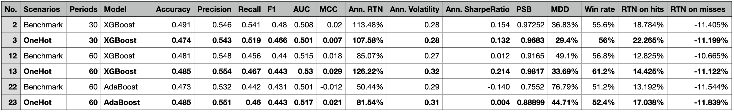
Stats benchmark summary of three scenarios
| XGBoost, 30 months | XGBoost, 60 months | AdaBoost, 60 months |
|---|---|---|
 |
 |
 |
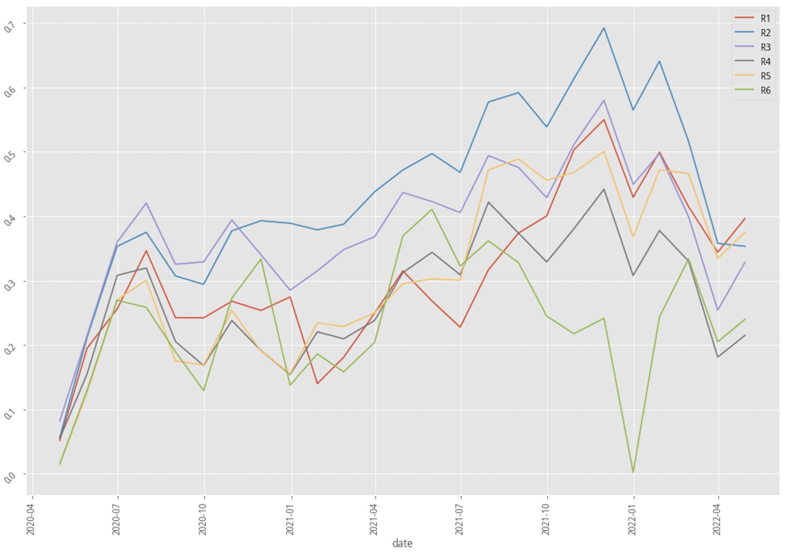
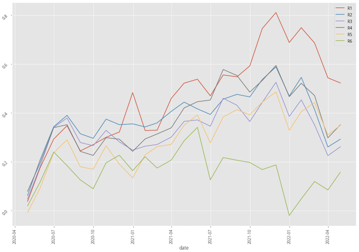
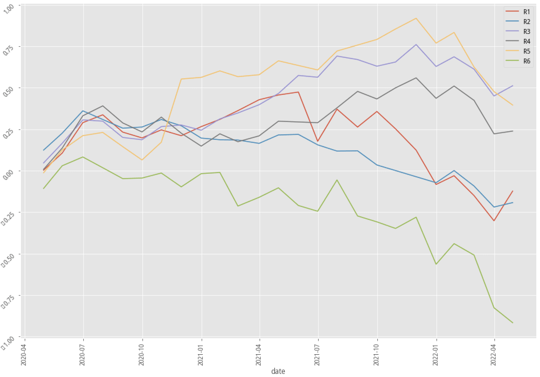
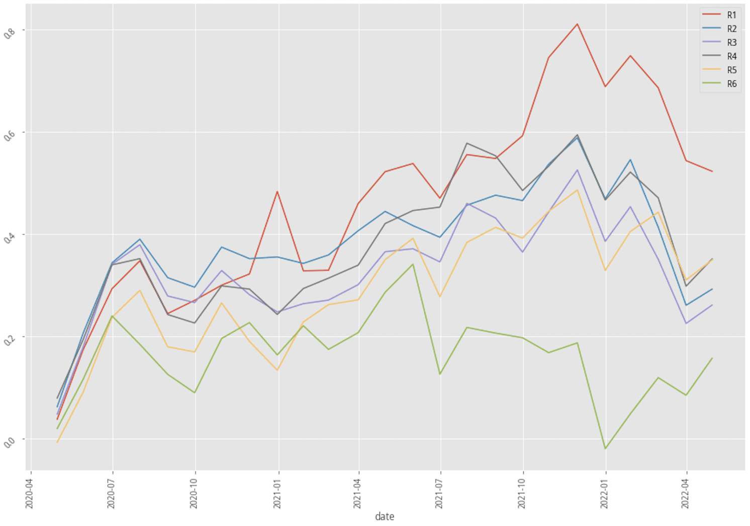
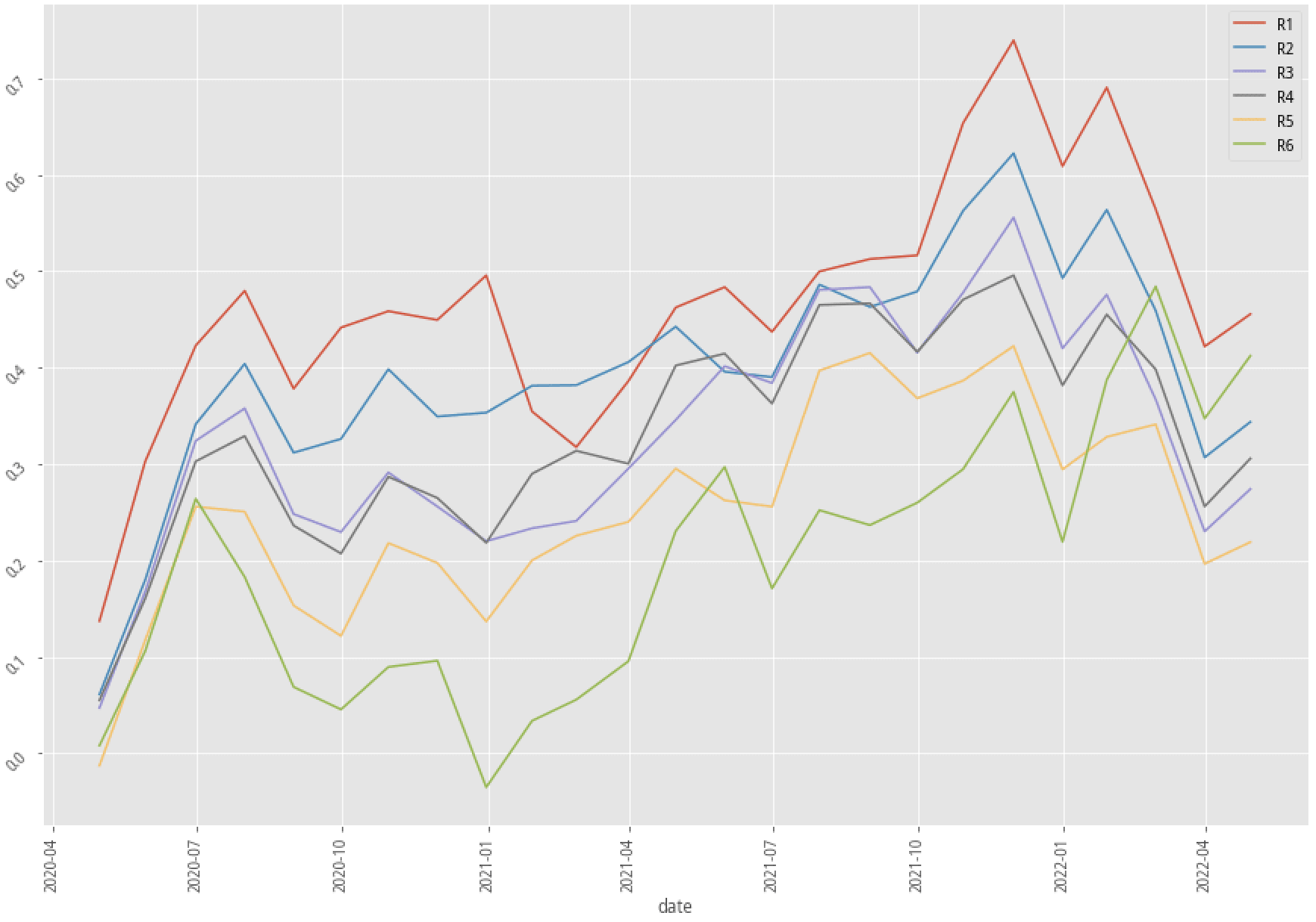
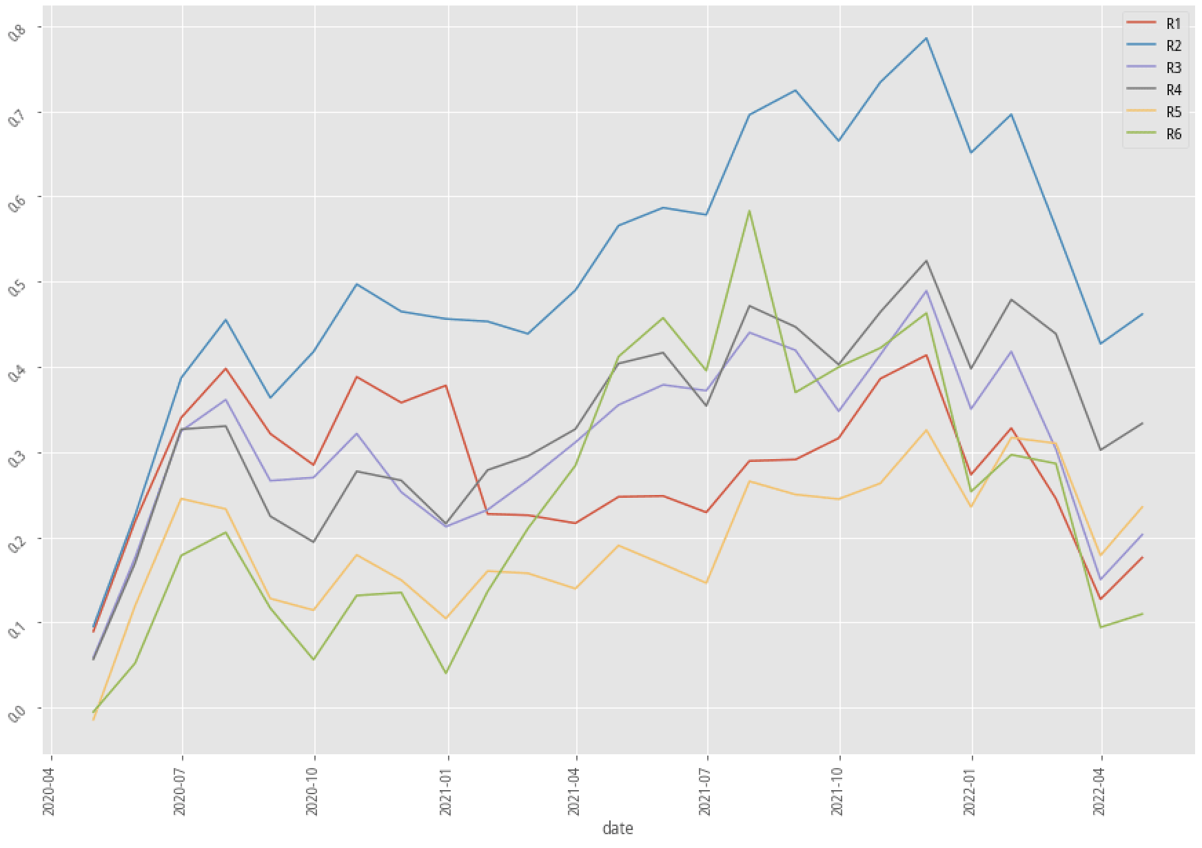
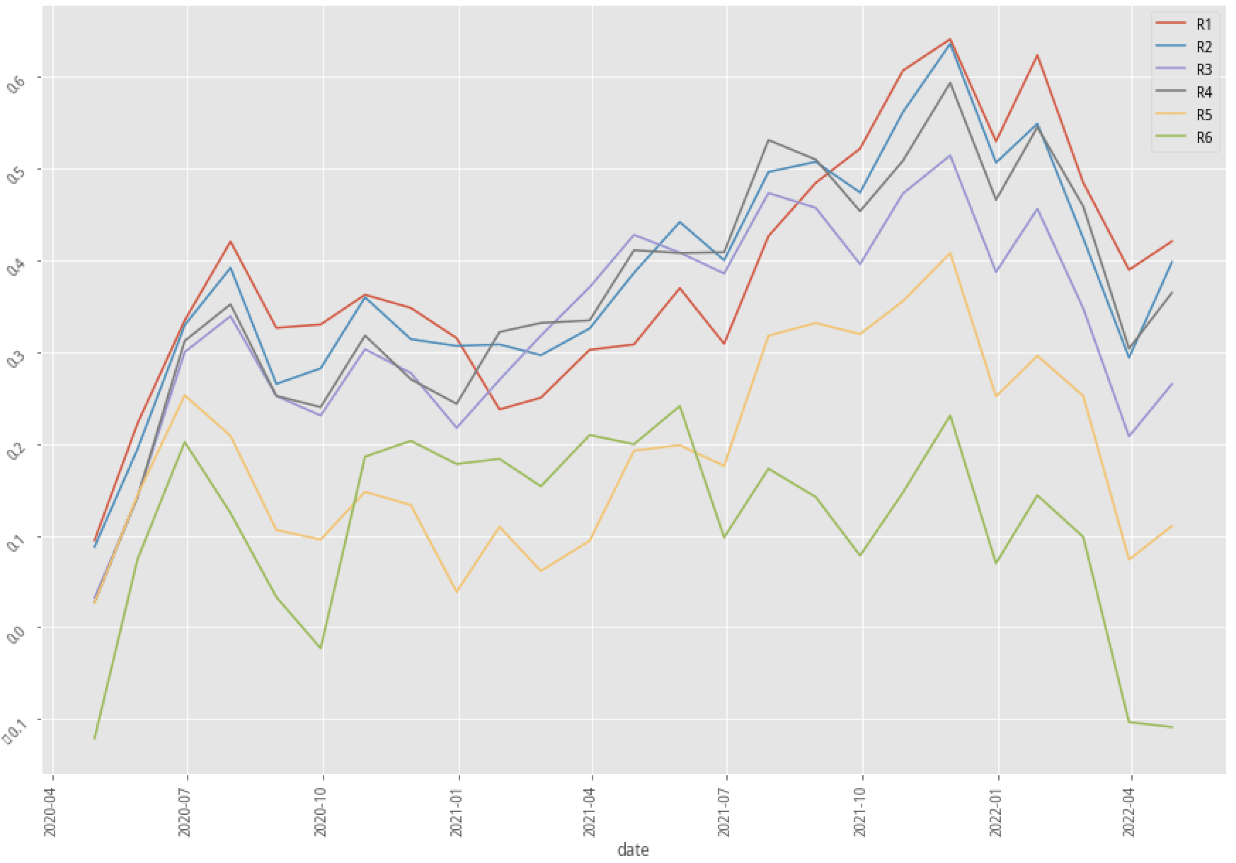
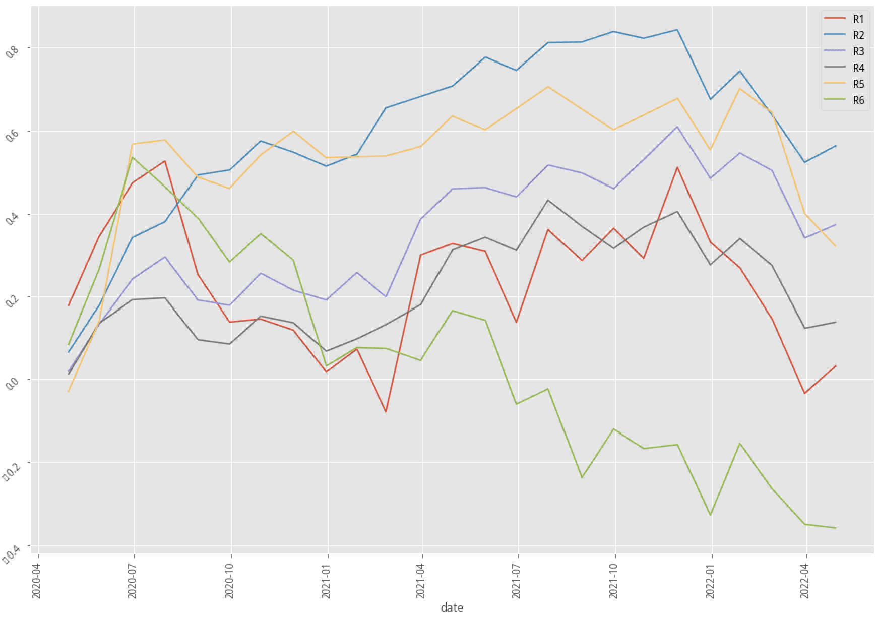
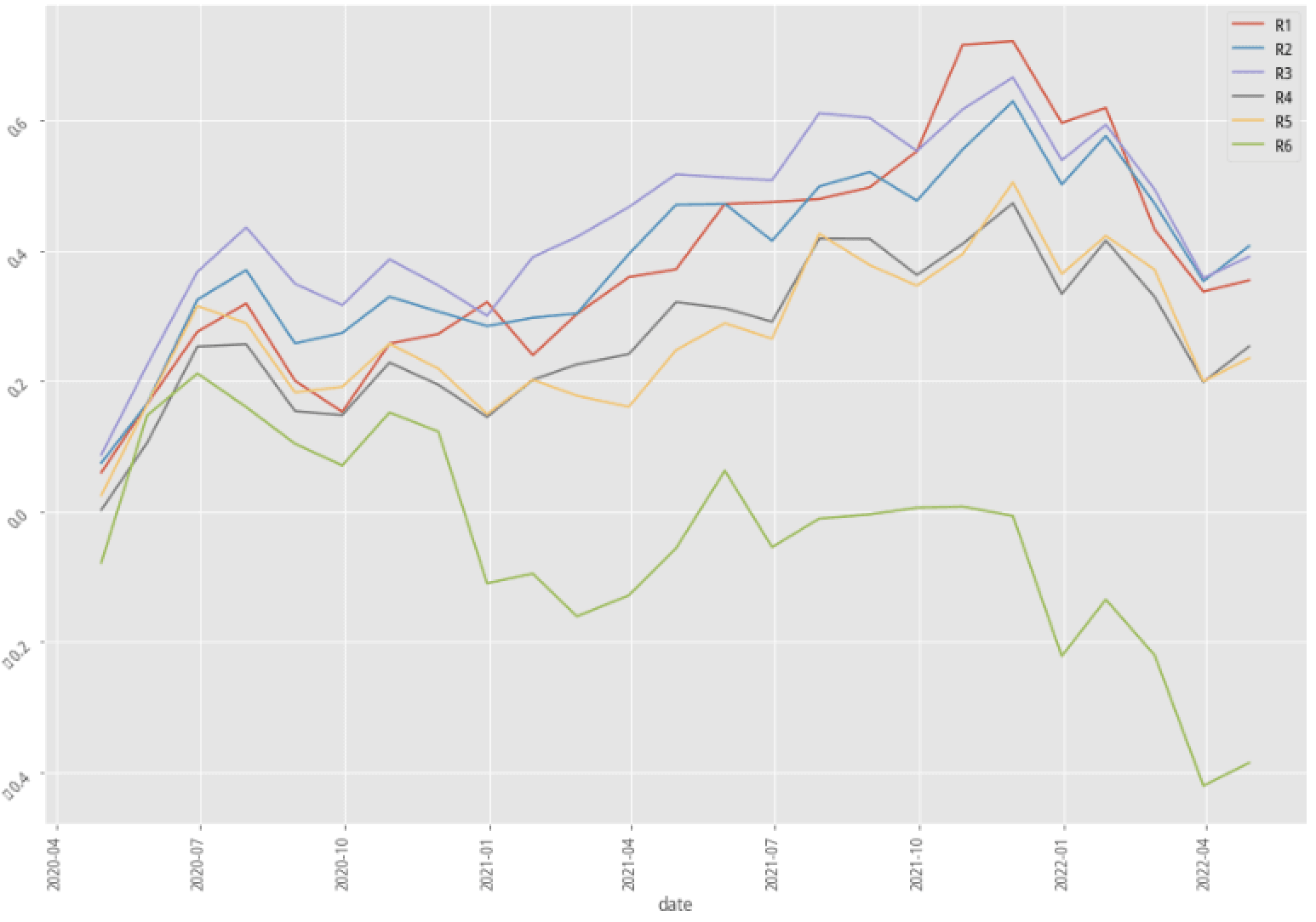
Stratified plotting of base scenarios return by probability to win
From the above table and charts, XGBoost with a 30-month data scenario is apparently the most lucrative scenario, and the scenario of using AdaBoost with 60-month data seems to work poorly compared to other scenarios. Now let’s first look at what could bring by adding industry feature to our feature set.
Adding industry feature - Encoding
Why adding industry feature
It’s a well-known fact that stocks in the same industry have similar wax and wane due to the reason that they are running a similar business, using similar materials, producing similar products, and providing similar services. It’s a common belief that this cyclical characteristic of stocks needs to be factored into our machine learning prediction model in order to reflect this phenomenon.
industry feature contains string-like data such as ‘Technology’, ‘Utilities’, or ‘Manufacturing’. However, both XGBoost and AdaBoost are tree-based classifiers that only accept ordinal numbers as features in training data. Therefore, we need to transform these string-like data into numbers so that our classifiers can understand the data.
One-hot encoding
The technique to transform string-like data into ordinal data is called encoding. Typically we apply Label Encoding, in which we use one number to label one string in the Industry column. One implicit drawback of it is that Label Encoding might suggest that the bigger number is more important than the smaller number. Taking the below table as an example, is {'Electric' = 4} really more important than {'Technology' = 1} in the transformed training data set?
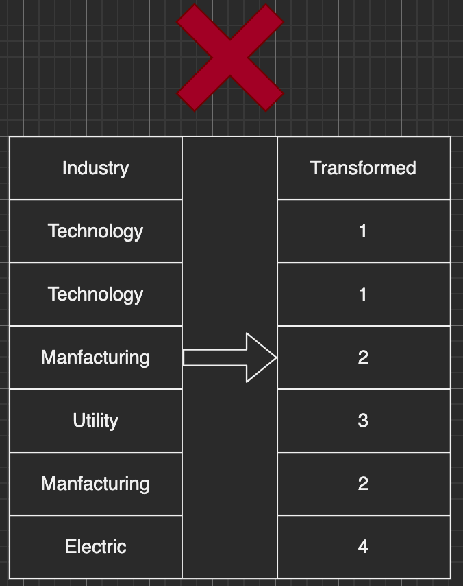
Label encoding doesn't work in this case
Here’s where One-hot Encoding comes into play. One-hot Encoding is a labeling technique that essentially uses one full column to present one single value in the original Industry column. The transformed data would have N new columns when there is N unique value in the Industry column. By doing this, we can remove the ordinal implication from Label Encoding.
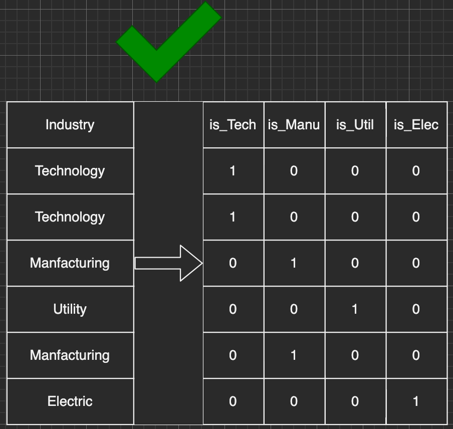
One-hot encoding transformation
Backtest results
Performance summary of three base scenarios with one-hot transformed industry feature
| XGBoost, 30 months | XGBoost, 60 months | AdaBoost, 60 months |
|---|---|---|
|
|
|
One-hot encoded |
One-hot encoded |
One-hot encoded |
 |
 |
 |
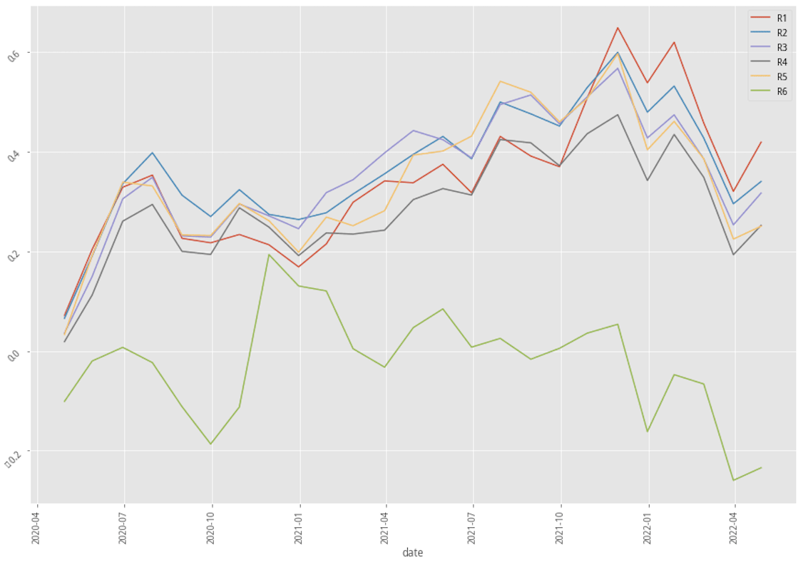
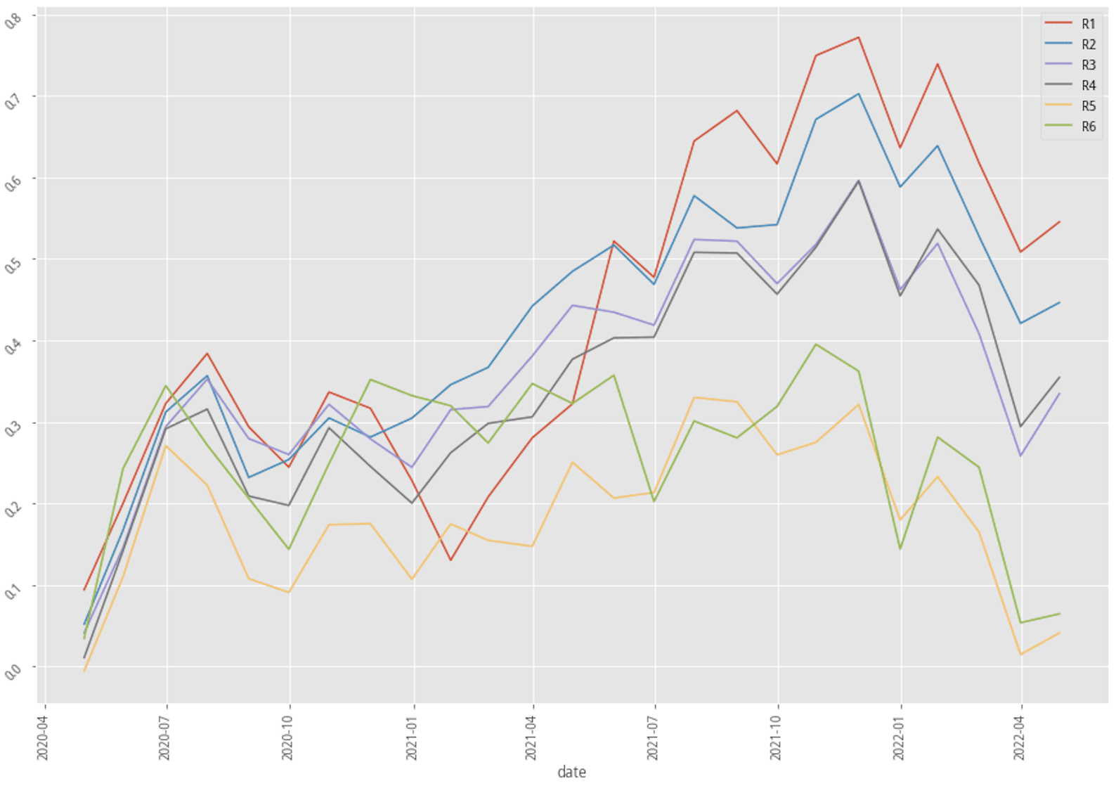
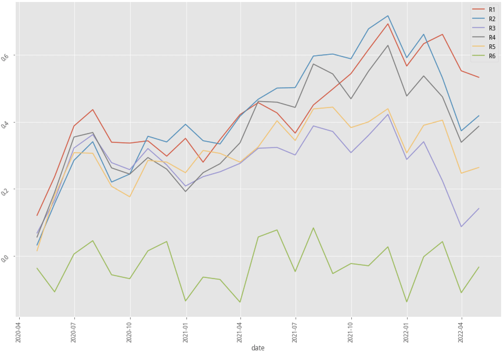
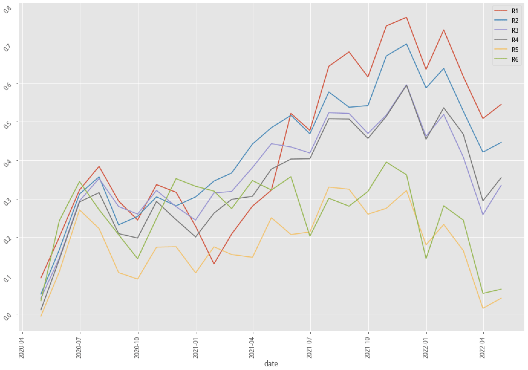
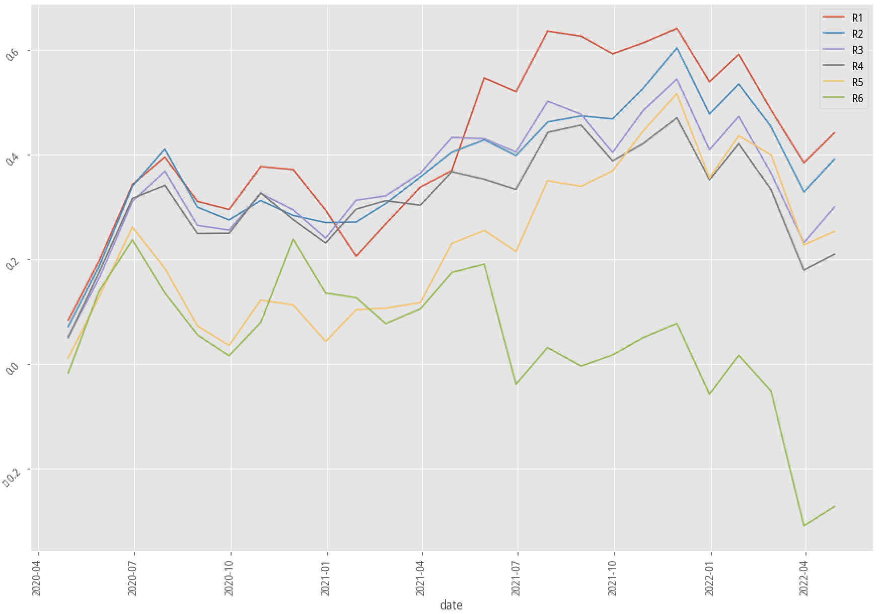
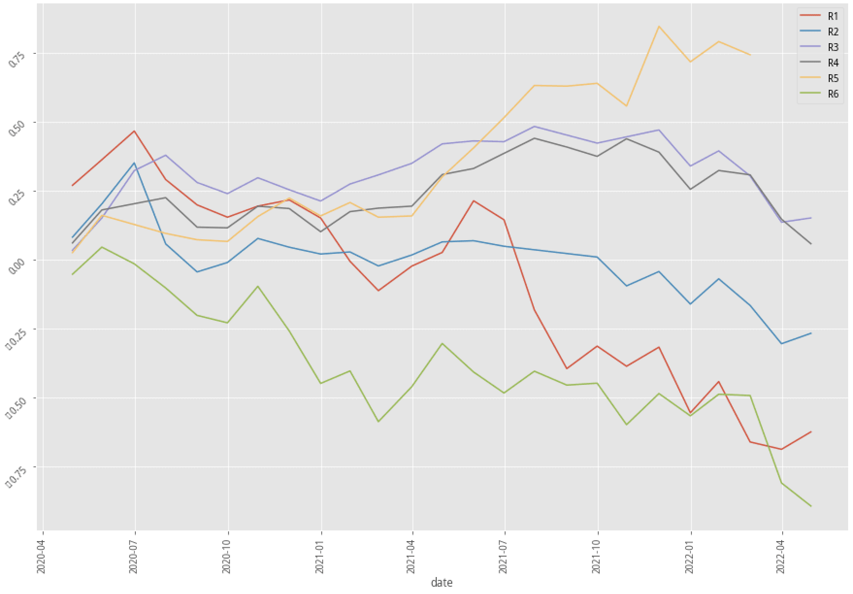
Stratified plotting of one-hot encoded enhanced scenario returns by probability to win
The performance of the two scenarios using XGBoost actually improved quite a bit in terms of the portfolio return, win rate, and even the Machine Learning score like F1, AUC, and MCC. These backtest results possibly suggest that accounting industry feature into our machine learning model does help generate a better-trained model.
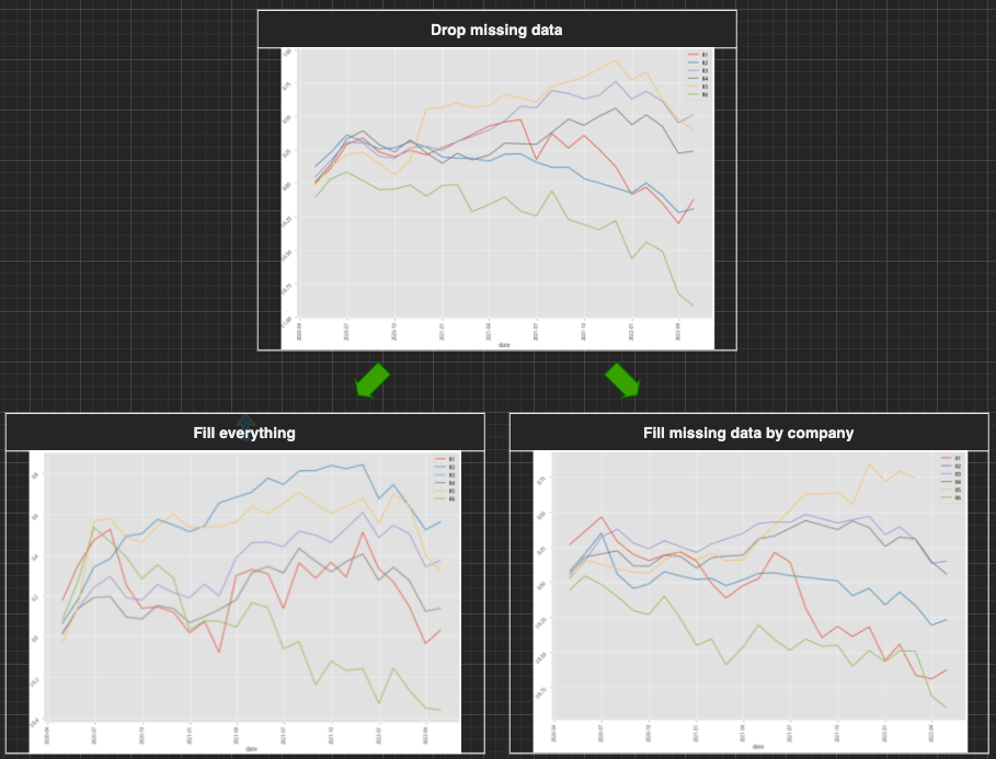
Dealing with missing data (NA) - Imputer
Previously in the post 【Machine Learning】 Part II - How to build a machine learning boilerplate?, the way we deal with the missing data is to drop all of them to avoid adding human-biased data. This is actually a luxury move for data scientists as the amount of the data is usually quite limited. If we can gently cast some fairy dust and revive those dumped data, the amount of data could be doubled or even tripled, and then train our model to be more accurate.

Imputer? What is it?
Imputer is a word actually found in sklearn machine learning python package, and the meaning of the word hardly tells me what it does. Imputer in sklearn is a sub-package to fill the missing data in various ways. There are SimpleImputer that fills the missing data with the mean of all the numbers, KNNImputer that separate data into different groups and fills the missing data with the mean of numbers in the same group, and also IterativeImputer that fills the missing data by estimation instead of the mean. In this post, SimpleImputer would be the tool that we’re using to fill the missing data.
Three scenarios to fill the missing data
Even though we’re using the simple SimpleImputer, there are still ways we can fill the missing data in a more sensible way.
- Drop all the columns that have missing data
- This is the original method how we deal with the missing data in our machine learning model. The missing data is dropped instead of filling any arbitrary number so that we don’t add any personal bias to the dataset.
- Fill all the data by column
- We fill every the missing data together so that all the missing numbers of the same feature will be filled in the mean of all available numbers.
- Fill the missing data by symbol
- In our training data, we have features such as company quarterly sales, gross profit, and cash/debt ratio(refer to Factor analysis Part III). These company-specific fundamental numbers can be very different from one company to another due to the nature of the industry or company itself. For example, company A quarterly sales are 1M, 1.5M, 2M in Q1, Q2, and Q3 respectively. On the other hand, the quarterly sales of company B could be 20B in Q1, 21B in Q2, but Q3 data is missing. It won’t make any sense if we fill the missing Q3 of company B with the mean of (1M, 1.5M, 2M, 20B, 21B), right? That’s why it is better we fill the missing data according to the existing data of the company itself.
Backtest results
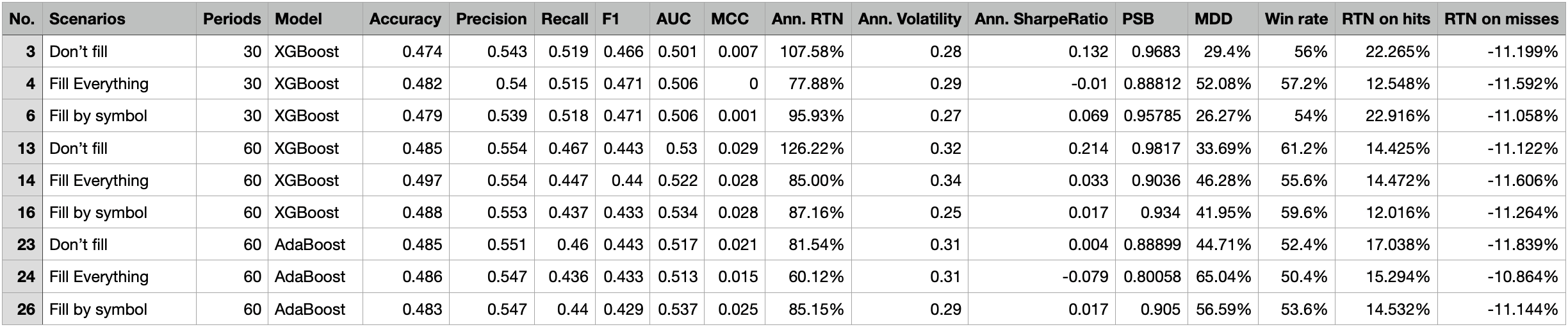
Performance summary of three base scenarios with imputed data
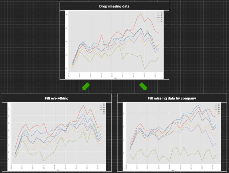
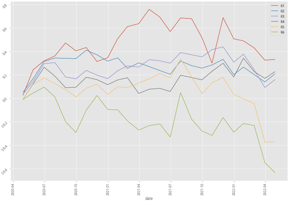
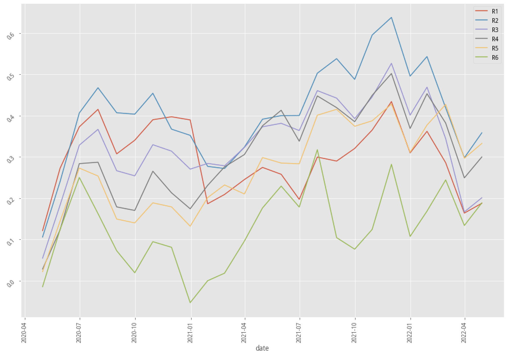
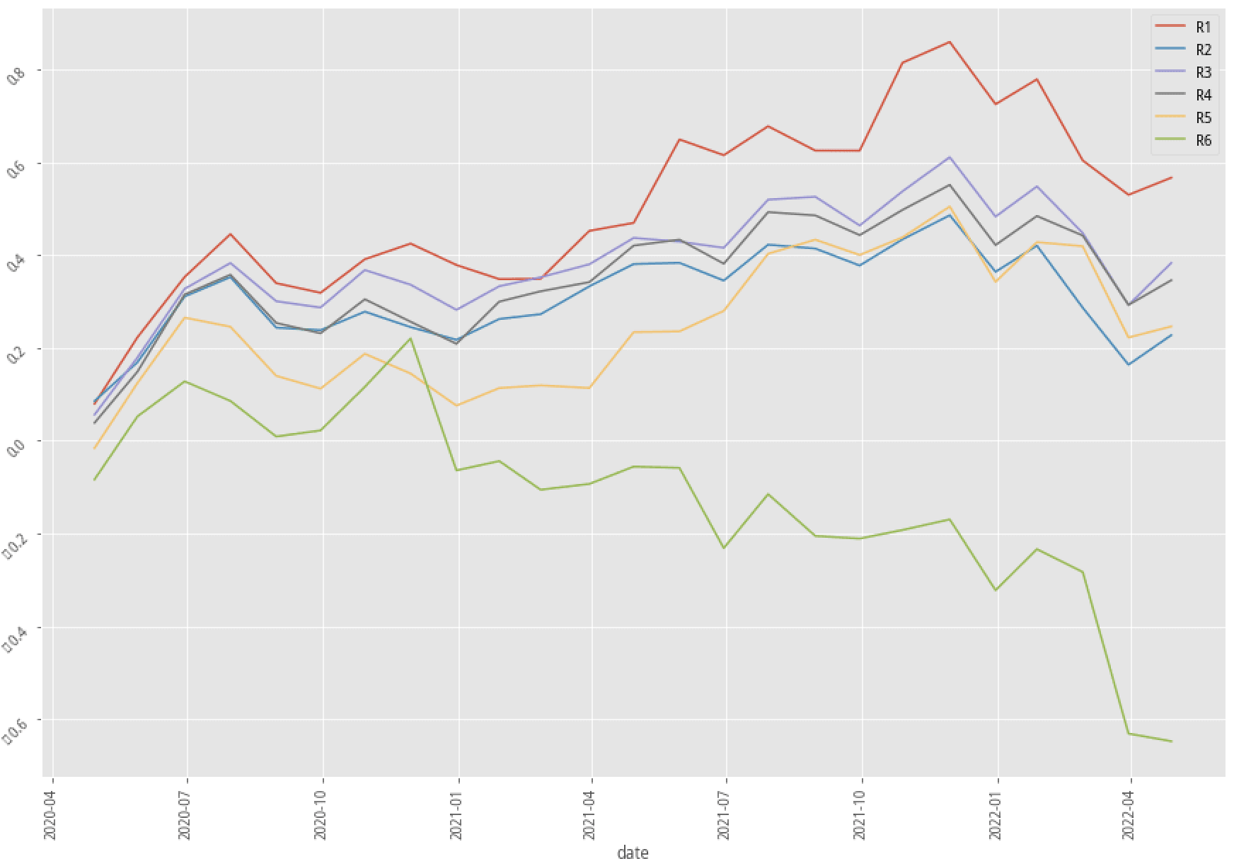
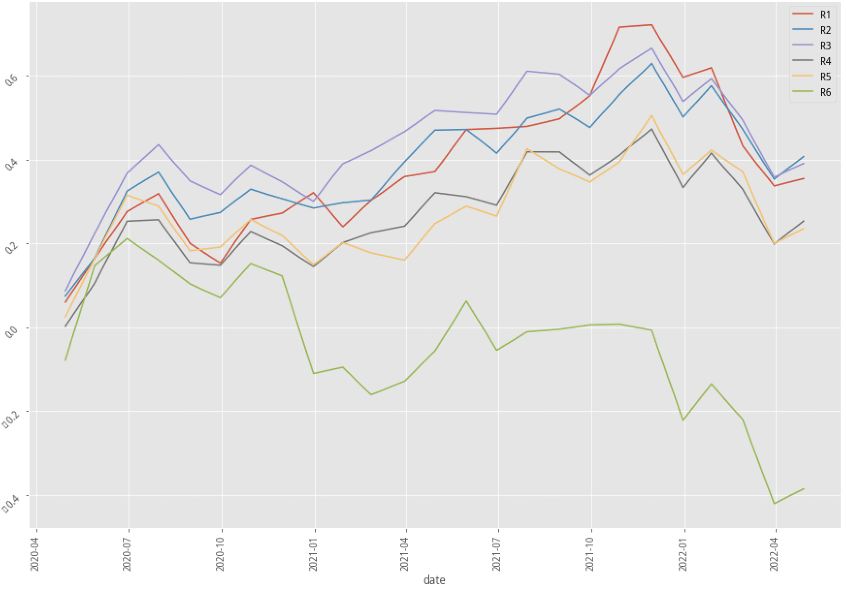
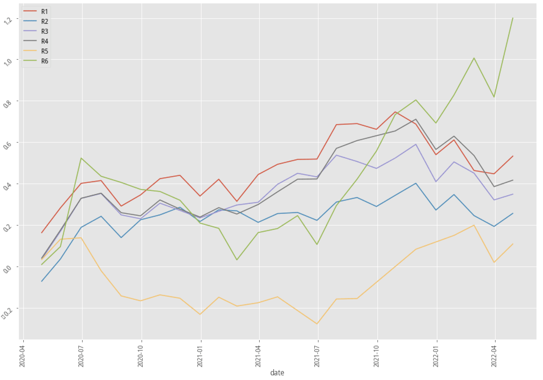
XGBoost, 30-month data performance stratified plot
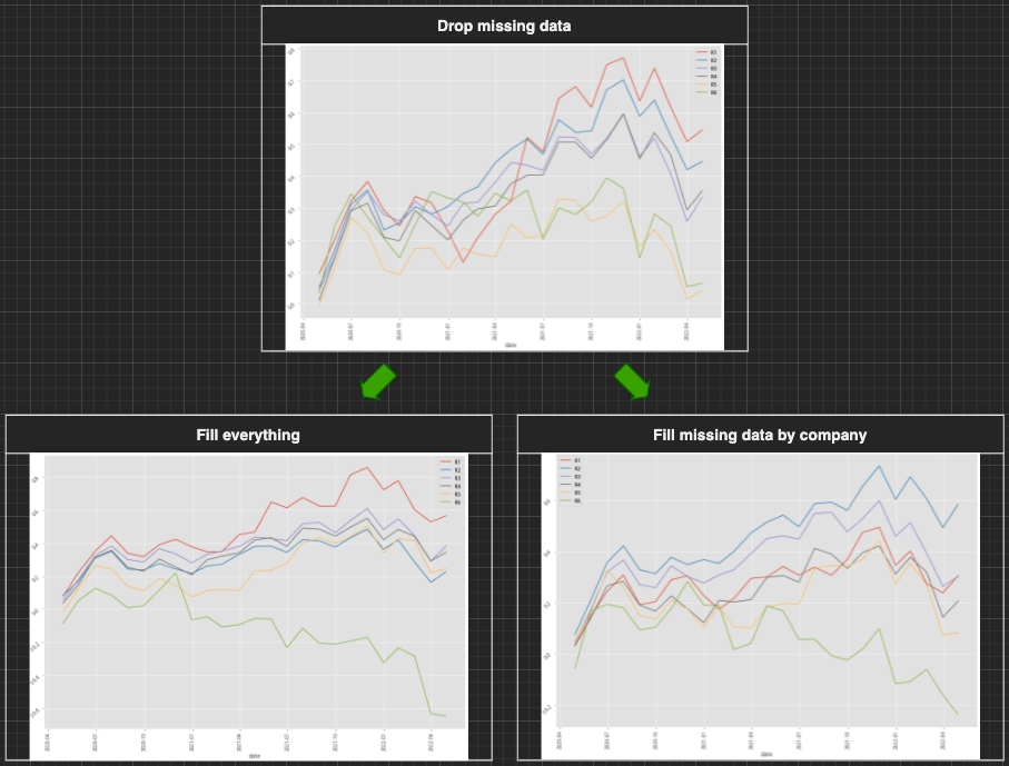
XGBoost, 60-month data performance stratified plot
AdaBoost, 60-month data performance stratified plot
From the first summary table, it’s quite clear that the performances of the data-imputed scenarios are worse than the performance of the drop-missing-data scenario. Not only the annual return dropped 20~30%, and also the win rate, MDD, MCC score, and other figures drop significantly compared to the benchmark scenario. Then we move on to the stratified plot of our three base scenarios. Either the fill-everything scenario or the fill-missing-data-by-company scenario has greatly contributed to the ability to effectively separate the most probable winning group (group 1, red line) from the other groups. We might now be able to extract and form our preliminary conclusion that "SimpleImputer" might not work in these scenarios but add more noises to the model, further decreasing the precision and accuracy of our model. You can also try out the KNNImputer or IterativeImputer to see whether can achieve a better outcome.
Combine features -> Kmean
What is Kmean and how to decide “K”
K-mean is a method/technique that aims to cluster all the data into K groups by analyzing the given features. I’m not going to go through the details and how to conduct your own k-mean clustering, as there are so many people doing so on medium and other ML platforms. I’m only going to reveal and illustrate the backtest outcomes to you.
What’s the benefit of conducting k-mean clustering? In the financial ML model, there are so many fundamental data such as sales, gross profit, and cash-to-debt ratio of every individual company. However, it’s a bit too complicated to take all these fundamental figures into account while training our ML model. Therefore, instead of using these fundamental figures as they were, it would be easier, more meaningful, and more effective if we can categorize them into several groups before we feed the data into the machine learning model.
Combining features
Let’s take the example that we used in our backtest, that we combine features ROA, asset turnover, Sharpe ratio since the last 20 days, and Sharpe ratio since the last 60 days. Instead of feeding these figures right into the machine learning model, we use the k-mean clustering method to categorize them into K groups and name the group feature profitability_of_the_company. Wouldn’t that make more sense for the model to know how profitable the company is rather than knowing the fundamental figures of the company? But remember, that the ordinal number is not suitable for the category type of data. Make sure you use One-hot encoding to separate the profitability type into features so that you’ll be able to feed these data into the model in a correct way.
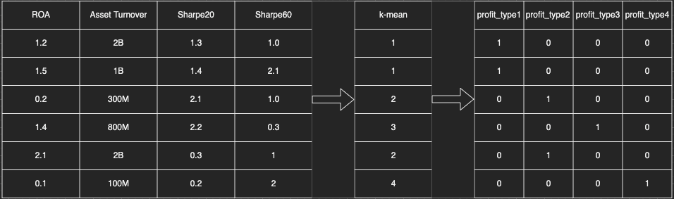
Using Kmean to produce meaningful features
Backtest results
Performance summary of three base scenarios with imputed data and additional kmean clustering
| Drop missing data | Impute everything | Impute missing data by company |
|---|---|---|
 |
 |
 |
Added kmean feature |
Added kmean feature |
Added kmean feature |
 |
 |
 |
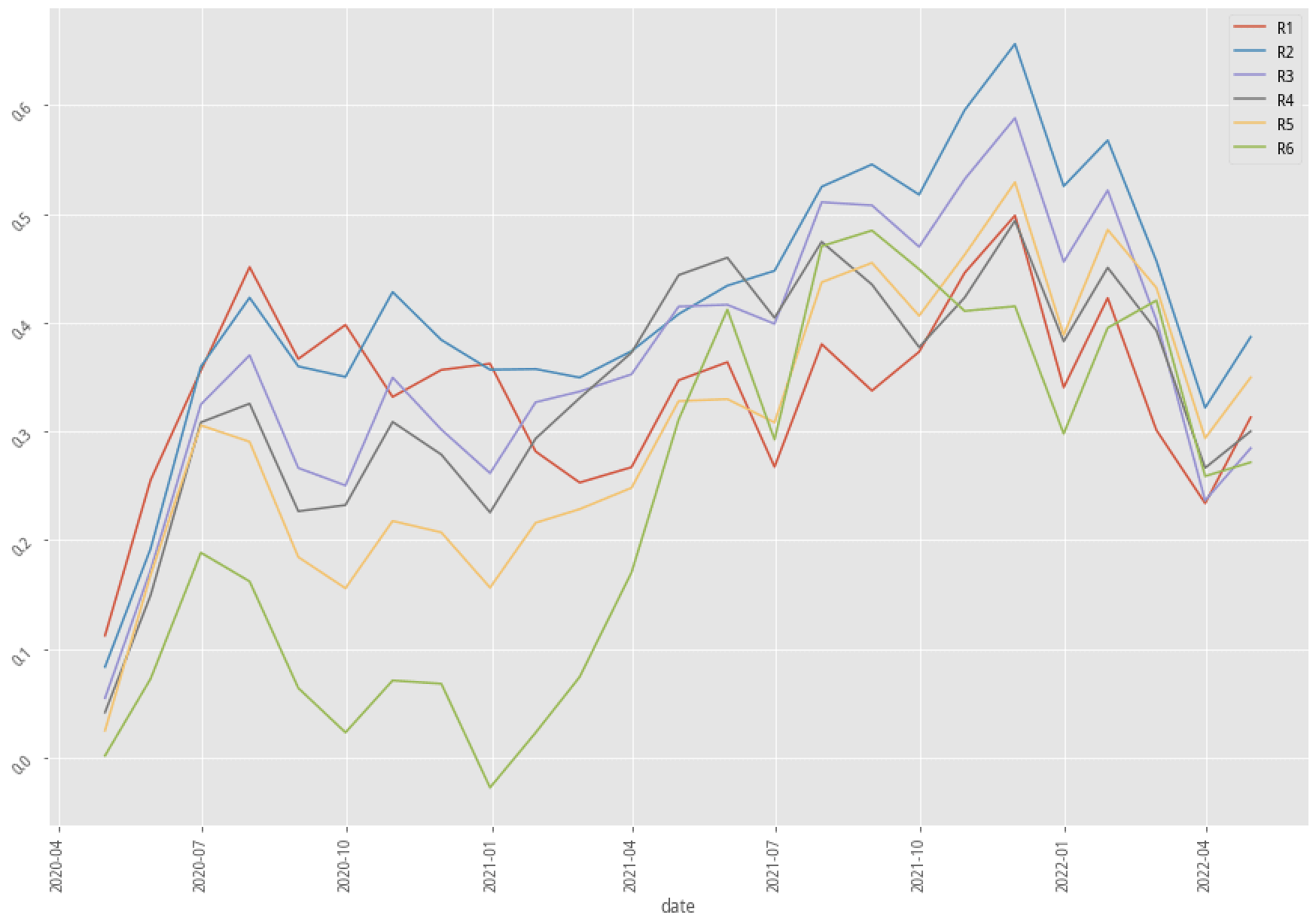
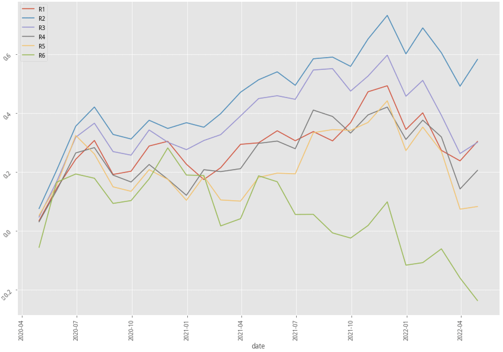
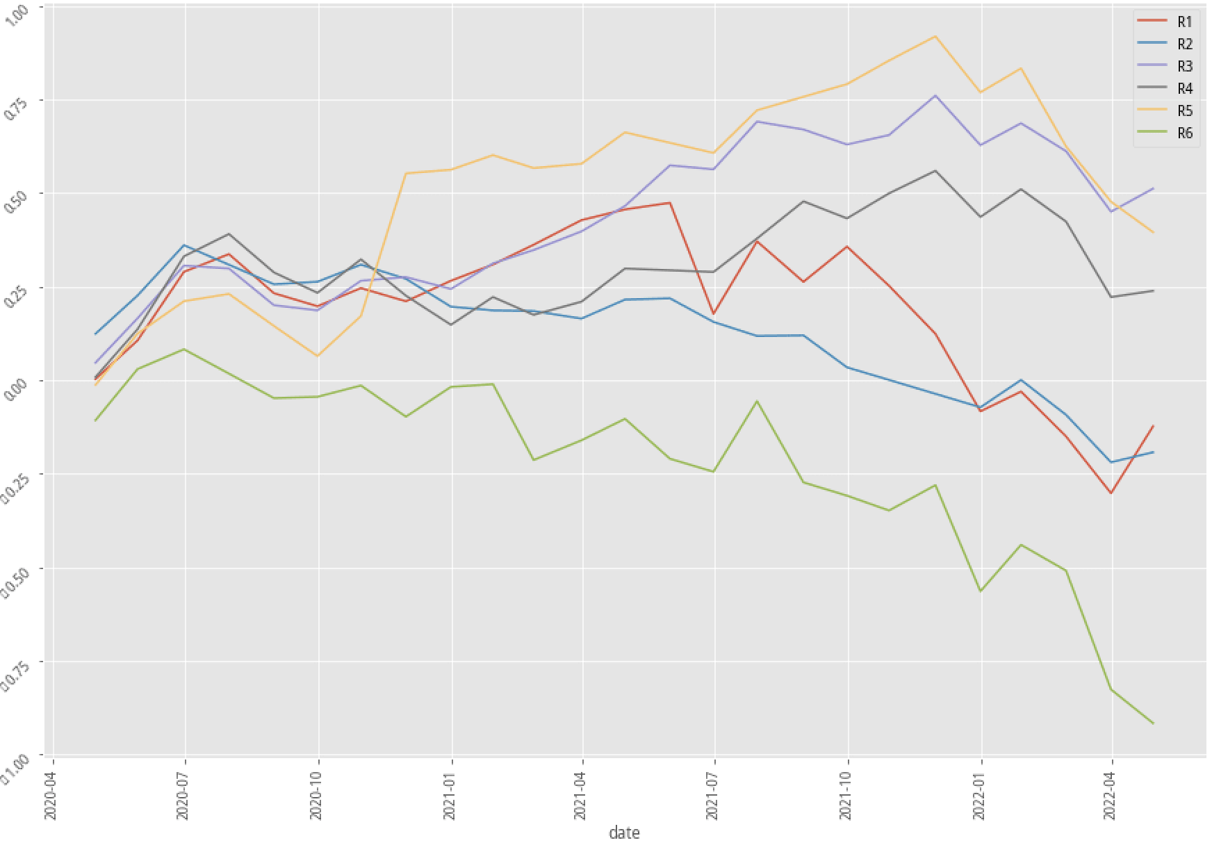
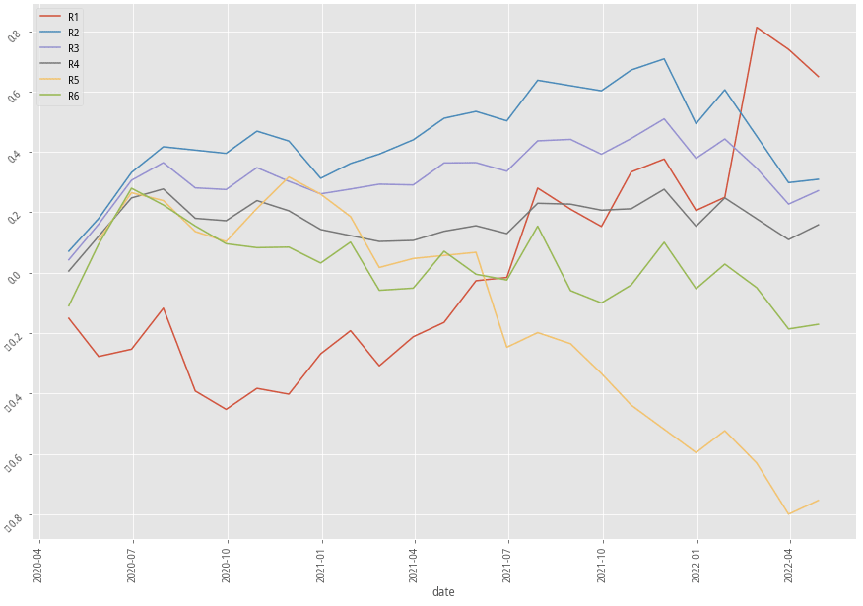
XGBoost, 30-month data performance stratified plot
| Drop missing data | Impute everything | Impute missing data by company |
|---|---|---|
 |
 |
 |
Added kmean feature |
Added kmean feature |
Added kmean feature |
 |
 |
 |
XGBoost, 60-month data performance stratified plot
| Drop missing data | Impute everything | Impute missing data by company |
|---|---|---|
 |
 |
 |
Added kmean feature |
Added kmean feature |
Added kmean feature |
 |
 |
 |
AdaBoost, 60-month data performance stratified plot
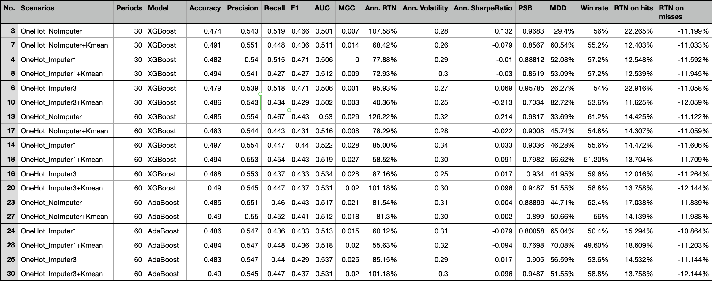
Again, let’s first look at the summary table. There are only two out of nine scenarios that have better annual returns after adopting the kmean clustering method. Our profitability_of_the_company factor doesn’t seem to be an effective way to raise the probability of win rate in the trading strategy. Fortunately, the experiment doesn’t have to stop right here. There are hundreds of features that we can test and try to see how to produce an effective, explainable feature that corresponds to our trading idea.
Conclusion
Among all three feature engineering techniques that we have adopted into our strategy, it seems that One-hot encodes the industry feature does enhance the predicting ability in our trading model. On the other hand, we can use KNNImputer as an alternative for SimpleImputer, and maybe try more combinations to create our new feature from the existing features.