
| Previous readings |
|---|
| 【Pair Trading】Introduction to pair trading strategy |
After knowing what the pair trading strategy is about from the previous post, we’re going to use the QuantConnect platform to research and validate each variation of the distance method. The agenda of this post would be:
- Introduction: what is the distance approach and what are its variants
- Research methodology: the methodology we use to conduct this research
- Research and performance analysis: Implement each variation and compare
Let’s get it started!

Introduction
The distance approach in pair trading was first popularized by Gatev, Goetzmann, and Rouwenhorst in their academic paper in 2006. This was because of its effectiveness of selecting the paired stocks that track each other well back then. Along with the simplicity in calculating the distance which saves computation resources, this academic paper became the most cited paper of pair trading strategy and derived many different strategies to further discover the relationship between stocks in the stock pair.
Basic distance approach
The basic idea of the distance approach is to use data in the formation period to calculate the Euclidean squared distances between each pair of normalized prices during the pair selection process. This Euclidean squared distance can be interpreted as the similarity of how do the stock normalized prices move in a defined period. The smaller the Euclidean squared distance of a stock pair is, the more similar movements these two assets have. Therefore, we’re going to pick the stock pair that has the smallest Euclidean squared distance as its spread should be stable enough to expect the spread will revert when rising to the peak or hitting the rock bottom.
The formula of Euclidean squared distance
Variants of distance approach
Other than using Euclidean squared distance to evaluate how two assets are correlated, there are other methods evolving from the basic strategy such as Pearson’s correlation, distance correlation, angular distance, and so on. Also, there are other additional ideas added to the distance approach to discover what is the best-fit stock pair to be traded. The following methods were introduced in the below papers: Gatev et al. (2006): Pairs Trading: Performance of a Relative Value Arbitrage Rule, Do and Faff(2011): Are Pairs Trading Profits Robust to Trading Costs?, Do and Faff (2012): Does Simple Pairs Trading Still Work?. These approaches are:
- Selecting pairs that are in the same industry group
- Selecting pairs with a higher number of zero-crossings
- Selecting pairs with a higher historical variance
- Selecting pairs with a higher Pearson’s correlation
Research methodology
To find out which one is the most effective method among distance approach and its variants, we have to set up a few rules to make sure that all backtests we are going to perform are tested under the same controlled environment:
- Use the constituents of the S&P 500 index as our universe, meaning we will consider only the stocks that are in the S&P 500 index.
- Take 12+12 months’ daily close price of each stock in our defined universe. Data from the first 12-month period was used to form/train our pair trading model, and then the following 12 months’ data were used to backtest the model against the real-world scenario.
- Normalize price data before we train our pair trading model. Let’s say we have stock A price ranging from \$100 ~ \$180, stock B price sits around \$20.00, and stock C price is over \$1000. The distances between pair A-B and pair B-C won’t be comparable because they don’t share the same starting point. Therefore normalizing price data removes the differences between two stock prices in order to make all pairs comparable.
- As there are 121,771 pairs been generated, we reserve the top 10% and drop the remaining 90% of the under-performed pair in order not to waste time to analyze the pairs that are not significantly correlated.
- Rank the stocks by the possibility of getting a positive return the next day (from high to low). The way to decide the possibility is different in every variant.
- We calculate and analyze the expected return from two different angles in order to evaluate which strategy is better:
6.1. Stratified analysis: Separate the stock pairs into 8 groups in order to see whether a higher possibility would actually result in a higher positive return.
6.2. Long strategy analysis: Take the first 20 stocks to calculate the expected return so that we won’t take in too many noises into our performance analysis. - Generate trading signals:
7.1. If the spread value exceeds 1.5 times of the historical deviations of the spread ($1.5\sigma$), generate a sell signal.
7.2. If the spread value drops below 1.5 times of the historical deviations of the spread ($1.5\sigma$), generate a buy signal
7.3. Close the open position when spread crosses over above or below the zero-line of the historical deviation.
Tips:
itertools.combinations()is a good util tool to create combinations contain two different symbols, for example('AAPL','AMZN')- Normalization formula: $P_{Normalized} = \frac{P - min(P)}{max(P) - min(P)}$.
- $min(P)$ and $max(P)$ are extracted from the formation period, and apply to the price data in backtest period
Research and performance analysis
Here we’re going to quickly talk about them and then we’ll conduct research and backtest against the basic distance approach and its variants.
Basic distance approach
Approach description
We calculate the SSD of each pair and take the top 10% pairs which have the smallest SSD to conduct the performance analysis.
Stratified analysis
Among 8 groups, group 1 contains the pairs that have the smallest SSD, and group 8 contains the pairs that have the biggest SSD. However, group 1 doesn’t seem to generate a positive expected return and group 8 doesn’t induce the relative huge loss as expected. The magnitude of SSD doesn’t seem to positively correlate to the expected return as we expect.
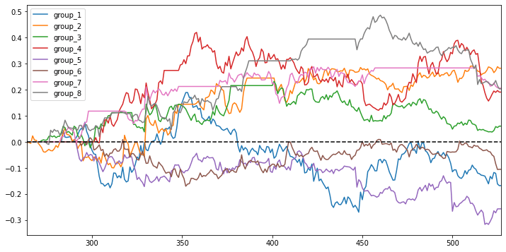
Basic distance approach stratified analysis
Long strategy performance analysis
If we long 20 the most stable stock pair by picking the pairs that have the smallest SSD, the portfolio still doesn’t generate a positive portfolio return over 12 months.
Basic distance approach long strategy analysis (Top 20 stocks)
Selecting pairs that are in the same industry group
This method holds an assumption that the paired stocks that are in the same industry are more likely to move together. So the idea here is to categorize each company by Morning Star sector code and pair the stocks within the same sector/industry group. Once we have these pairs from the same industry prepared, then we do exactly the same as the basic distance approach in order to analyze the portfolio performance.
Stratified analysis
It’s still a mess. Our group 1 that suppose to make the most profit actually incurred the most loss. The lines that represented the accumulated return of each group tangled tightly instead of staying apart from each other.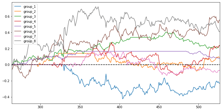
Same industry distance approach stratified analysis
Stratified analysis by sector
One more analysis we can do is to see which sector performs the worst. The sectors that perform the worst are 101 and 206, which are the Material and the Health care sectors. Therefore by conducting the stratified analysis by sector, we could potentially initiate another strategy by removing the sectors that perform worse in the first place.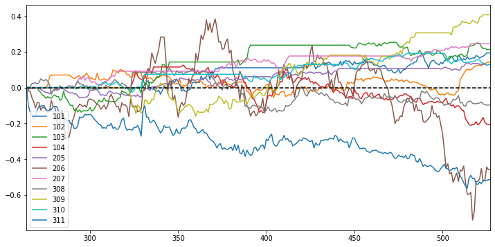
Expected return by sector
Long strategy performance analysis
It’s quite interesting to tell the line is very similar to the expected return above, meaning the top 20 pairs we picked could highly resemble the top 20 pairs in the basic distance approach. In terms of return, nothing gets improved. But one thing to be noticed is that by creating pairs within the same industry, we reduce the total pair from 121,771 pairs to 13,207 pairs and greatly reduce the time needed for the calculation.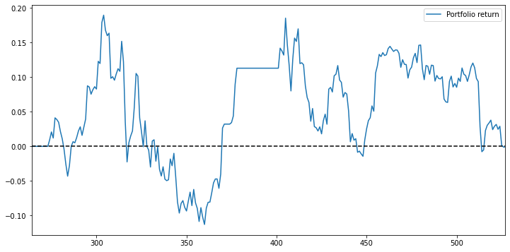
Same industry distance approach long strategy analysis (Top 20 stocks)
Selecting pairs with a higher number of zero-crossings
It’s a good sign that the spread of the paired stocks is stable enough. However, if the spread of a certain pair is way too stable, there will be no chance for the traders to step in and make a profit. Therefore in this variant, among the top 10% pairs that have the smallest Euclidean squared distance, we further pick the pairs that had the highest number of crossing the zero-spread line. A high number of zero-crossing gives this pair enough energy to swing up and down, but without losing the ability to maintain its stability and come back to the zero-spread line.
Here’s a tip to share with you, that it’s fairly simple to calculate the number of zero-crossing if you have your spread in proper time-series format.1
2
3# Both price_a and price_b are nd.array or pd.Series objects
spread = pd.Series((price_a - price_b).reshape(-1))
num_of_zero_crossing = ((spread * spread.shift())<0).sum()
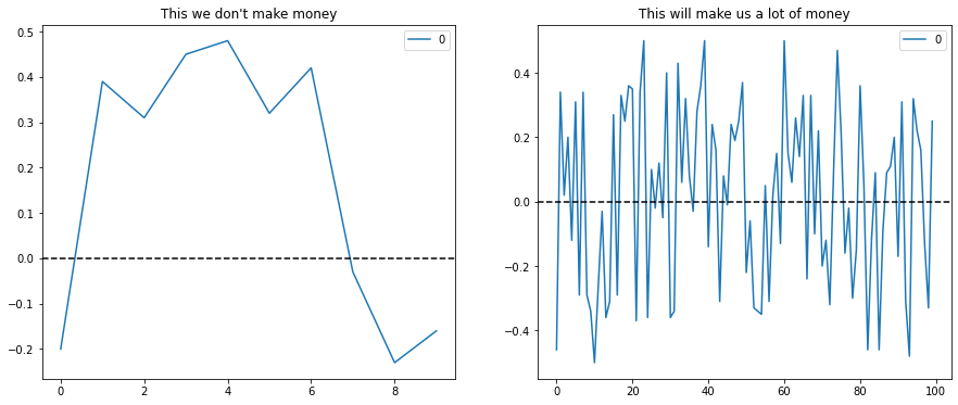
Why the number of zero-crossing matters
Stratified analysis
Now we do see the differences by adding the zero-crossing criteria. The first two groups that have the highest number of zero-crossing did stand out in the accumulated performance. However, the expected return of low zero-crossing pairs doesn’t tell us that we can count on this to form a market-neutral strategy. Maybe a long-only strategy would be better off.
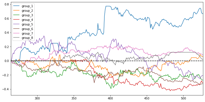
Zero-crossing distance approach stratified analysis
Long strategy performance analysis
It does! THe long-only strategy definitely helps gradually accumulate our portfolio return. This diagram kind of proving our assumption that the high value of zero-crossing would single out the pairs that are more resilient and are capable of reverting back to the normal spread level.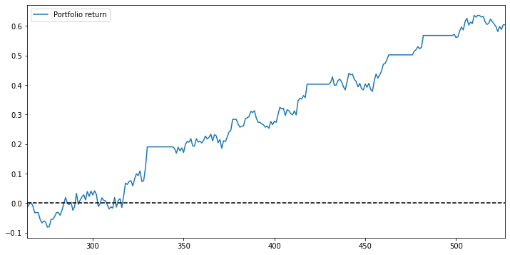
Zero-crossing distance approach long strategy analysis (Top 20 stocks)
Selecting pairs with higher historical variance
This variant actually used the same idea as above Selecting pairs with a higher number of zero-crossings. Instead of using the number of zero-crossings, this method takes the high variance as the sign of the spread between the paired stocks being fluctuated enough to be traded.
Stratified analysis
Um…. Don’t even bother talking about this diagram. This result obviously tells us that this variant is not a fit for market neutral strategy.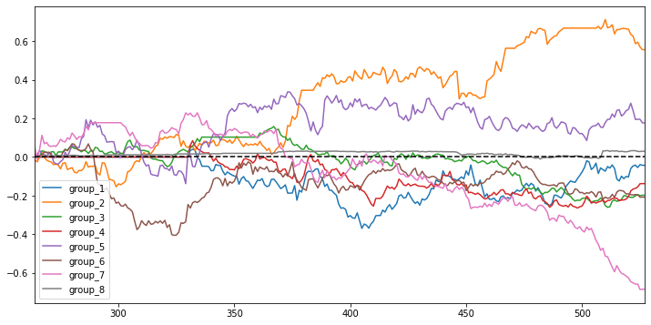
High variance distance approach stratified analysis
Long strategy performance analysis
Even though the accumulated return looks weaker than the return from the high zero-crossing long strategy, we still can expect this long-only strategy to perform well.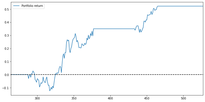
High variance distance approach long strategy analysis (Top 20 stocks)
Selecting pairs with higher Pearson’s correlation
This method is relatively more complex than the above methods. This variant is mentioned in the paper Chen et al. (2012): Empirical Investigation of an Equity Pairs Trading Strategy, and the paper Christopher Krauss (2015): Statistical arbitrage pairs trading strategies: Review and outlook.

One tracks a group of assets instead of tracking just one
The idea of this method is that we’re going to use the composition of 50 stocks as the benchmark to calculate the spread against the target asset. In this way, we’ll be able to diversify the specific risk by comparing it to a basket of stocks. To do this, we will need to use Pearson’s correlation to pick out the 50 most related assets to construct the benchmark portfolio of the target asset. Then instead of using historical deviation ($1.5 \sigma$) as the threshold to trigger our trading signals, we use linear regression to construct the relation between two stocks and then use calculated $\alpha$ and $\beta$ to calculate the deviation. The higher the number of the deviation, the more likely deviation will revert.
$where$
$R_{jt}$ is the return of the pairs portfolio
$R_{it}$ is the stock return
Stratified analysis
This time we do something easier. We pick the top 20 stocks that deviate the most from its benchmark portfolio and long them and pick the bottom 20 pairs that deviate least and short them.
This would be the perfect variant to formulate both the market-neutral strategy and the long-only strategy. The return of the stocks we long go straight up and the return of the stocks we short go down. In the meantime, both lines are negatively correlated. When the green line drop below the bottom and break through the zero lines, the red line (the return of the stocks we short) revert and recover the loss from the green line. By longing the top 20 and shorting the bottom 20, we perfectly form the market-neutral strategy that still makes a positive return over 12 months including the bear market.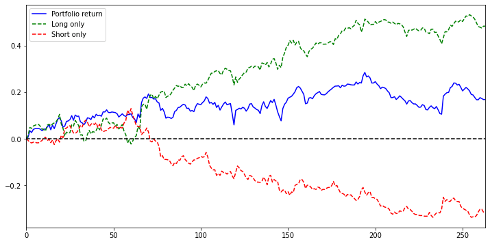
Pearson's correlation distance approach market neutral strategy
Final words and next step
Through the above researches, you can tell that the pair trading strategy is consist of four parts:
- Pair selection
- Model formation (to form $\sigma$ or benchmark return in Pearson’s correlation variant)
- Monitoring the current stats
- Generate trading signals against the trained model
The most important part I believe would be the pair selection part as I believe it’s crucial to find the pair/stock that does bounce back when the spread/price hit the ceiling and the floor. So essentially it’s still considered a mean reversion strategy.
Even though we have found our perfect strategy among these five variants, there are many things that we haven’t looked at such as:
- Should we use the rolling window to constantly update our model?
- Should we trade more than 20 stocks at a time?
- Should we find some other formulas to replace the Pearson’s correlation in order to find the more correlated paired stocks?
- Should we expand the whole universe instead of only looking at the stocks in S&P 500?
These can be the potential improvements that can be experimented with. Also, make sure you run the proper backtest using the backtesting platform as QuantConnect or JointQaunt to make sure you validate your algorithm against the real-world scenario.