【ML algo trading】 III - 5 myths about practicing quant trading with machine learning

In the post 【Machine Learning】 Part II - How to build a machine learning boilerplate?, we have successfully built our machine learning boilerplate. By having this template, we can develop an advanced machine learning trading strategy upon. However, even with the strategy result that looks profoundly profitable, we still won’t be able to know how much money we can make by looking at the accuracy rate of our machine learning trading algorithm.

In order to better understand whether the results from the output of our model are really concerning our portfolio return, I put together a rather simple strategy and run several backtests with different parameters. In the end, we’re going to answer several frequently asked questions in order to decrypt the myths of machine learning trading algorithms.

Here I introduced the JoinQuant platform into our toolset in order to backtest our strategy. After several times of tuning and research to further advance our preliminary machine learning boilerplate, I’ve executed 108 backtest on the JoinQuant platform to see how well the strategy could perform if we launch this machine learning strategy to the stock market. By summarizing the results from these 108 backtest, there are a few things that are interesting for beginners of quant trading to learn before developing their own machine learning quantitative trading strategies.

Setup before we start

Quick introduction of the machine learning models

I picked three different machine learning models to see whether different models will greatly impact the outcome of the strategy. Three models are: Logistic regression, SVM with Gaussian kernel, and XGBoost. I’m not going to cover the theory of each model as our focus in this article is to extract some valuable insights from the backtest results.

Logistic Regression

Logistic regression is one of the most commonly used algorithms in the field. Similar to the theory of linear regression as we explain Supervised Learning here, the input data will be fed into the pipeline to produce a final score. Logistic regression simply applies the Sigmoid function to convert the final score into either 0 or 1. We’re going to get an array of [1, 0, 0, 1, …, 0] as the outcome from the logistic regression, which we can reinterpret the array into [True, False, False, True, …, False] as our final results.

In other words, we’re trying to find the exact line to separate the 0’s and the 1’s.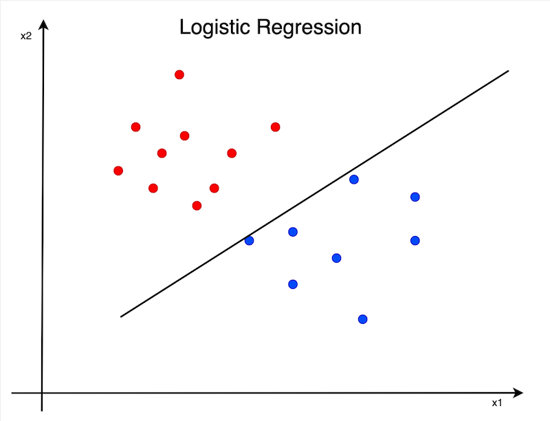

The classic linear regression model

SVM (Support Vector Machine)

SVM is a variant of logistic regression. Instead of finding the exact line to separate all the 0’s and the 1’s, we’re adding a buffer parameter (the penalty term C in the diagram) into the model. By adding this buffer, the model would be much more resilient to the test data.

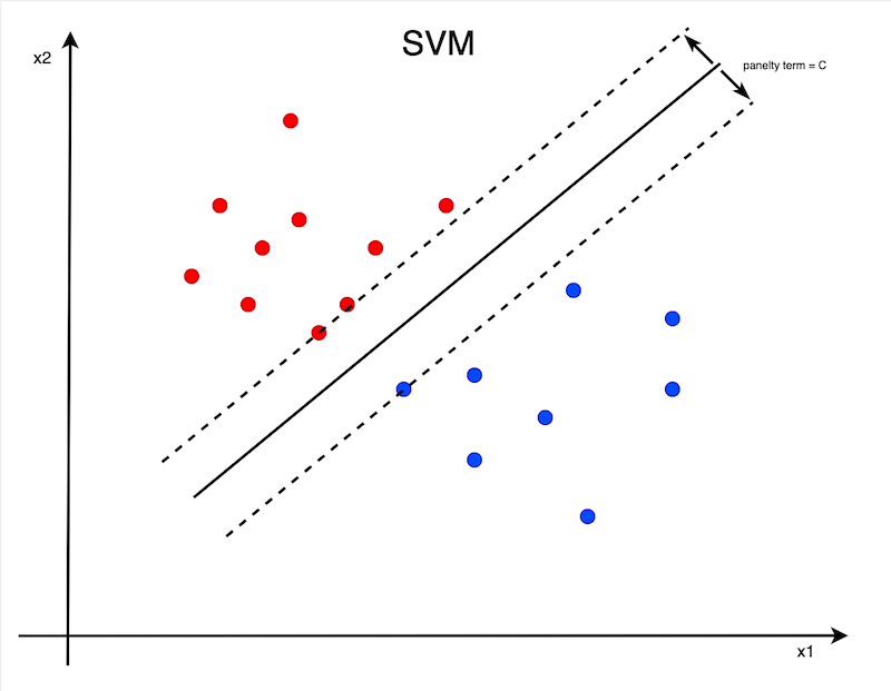
SVM is a more flexible classification model

XGBoost

XGBoost is a tree-like classification model. By inputting data into the tree-like trained model, the model will generate relative scores in each end leaf. After adding up all the scores presented in the leaves and applying the sigmoid function, we will have our final prediction for that specific test data. Essentially, it’s a different technique than the previous two algorithms.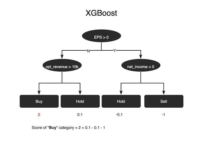

XGBoost is essentially a type of decision tree

Data and factors

Below are the data and factors that I used to train the model. You can reference here to know what these factors stand for.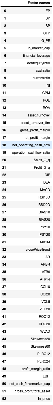

Factor data

Also, I neutralized the data against the industry category and market capitalization, and winsorized the data to mitigate the extreme data as standard steps to process the data.

How to train the model

I’m going to train the data as we said in this article. I didn’t split the CV data from the original data, as our purpose is to train the model constantly with the latest data instead of using the same batch of data over and over again. Standardization and Principal Component Analysis (PCA) were also applied to the data before training the model.

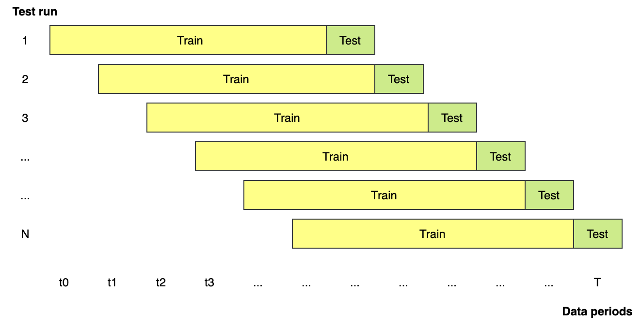
Rolling over the data to include new data and exclude old data

Our strategy

Let’s quickly put together our trade strategy to be used in this backtest experiment:

1. Collect and adjust our portfolio on monthly basis.
2. Label the stocks that have the top 30% daily return as +ve data, and the stocks that have the bottom 30% as -ve data. This label is what we used in the y_data to train our model.
3. Portfolio capacity set to be 20, meaning we can hold at most 20 stocks at the same time.
4. There are two variants regarding how to pick the stocks we’re going to buy:
   4.1. Buy the top 20 stocks that have the highest probabilities to be +ve.
   4.2. Buy the stocks that were predicted +ve.
5. We set our stop-gain point at 70%, and stop-loss point at 8%. 70% of stop gain would not stop us from gaining the margin of the top 30% stocks, and 8% would simply be my personal risk-aversion level.

Resolving myths

These 108 backtest were conducted with the test data from 2019-09-29 to 2021-05-07. The parameters include: the types of machine learning algorithms, the length of training periods, the number of selected factors, when to place orders, … etc. The benchmark is the ZZ500 index, and the benchmark return during the test period is 28.74%.

To show you what the result would be like, I screenshot one of the backtest results: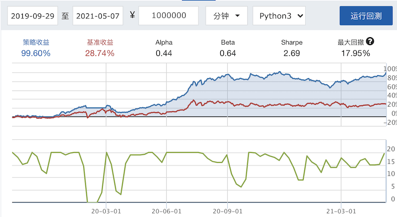

Backtest results ran on JoinQuant

However, it’s still quite difficult to find out what is the best case that has all the parameters right simply by looking at the numbers and chart. Here I put all the data into one CSV sheet and visualized the data to extract a few insights from different angles. Hopefully, we can get an idea of what are the most crucial parameters that we need to consider before we throw this strategy into the market. They are:

• Which of the machine learning algorithms has better performance?
• How many features we should use?
• How much data we should use to train our model?
• When should we trade our target stock?
• Is AUC the indicator we use to evaluate our model?

Which of the machine learning algorithms has better performance?

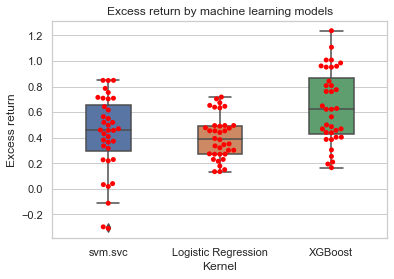
Excess return by machine learning models
The red dots indicate the excess return compares to the ZZ500 benchmark return of 28.74%

The LogisticRegression from sklearn.linear_model seems to have the most stable excess portfolio return ranging from ~15% to ~70%. XGBoost seems to be the best model as it gave us the best potential portfolio return ranging from 18% to 120%. As for the svm.svc (support vector machine model), which has too much downside risk and could potentially cause us to lose money, would be the least desirable model to utilize at the first glance.

How many features we should use?

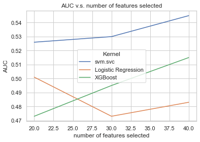
AUC v.s. number of features selected

I’ve run the backtest with 20, 30, 40 features using function RFE (Recursive feature elimination) in sklearn.feature_selection, which will analyze the features and then select the most relevant features. By looking at the diagram, you can tell that except for the Logistic Regression model, the higher AUC you will get if you picked more features to train your model. That might indicates that our model is capable of predicting more accurately if more features were accounted for.

AUC: AUC is the model evaluation indicator ranging from 0 to 1, which is used to evaluate the accuracy of your classification model. When 0.5 < AUC < 1, you actually own a pretty good machine learning model that classifies True or False.

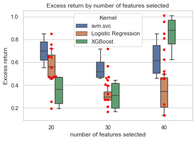
Excess return by the number of features selected

There is no clear increase of excess return even though we have higher AUC when you look at the above diagram. The red dots of excess return are dispersed all over the chart. The distribution of red dots is even more separated if we picked 40 features. This phenomenon potentially tells us that our model is over-fitting with 40-feature data, rendering a lower ability to predict the future. On the other hand, if we look at the scenario of XGBoost model with 40 features, this is the scenario that gives us the highest excess return with tolerable variance. So this could be one of our parameter combinations to apply to our final model.

How much data we should use to train our model?

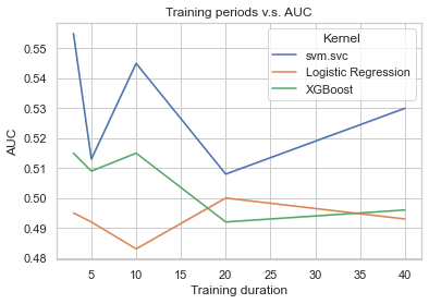
Training periods v.s. AUC

Machine learning is an algorithm that aggregates historical data to form a pattern and further uses this pattern to predict the future. The more data you feed into the model, the algorithm will have much more ideas to decide whether a specific scenario will happen or not. However, this doesn’t 100% apply to the stock market as there are too many variables and events that cannot be quantified as inputs to feed into the model. Also, stock prices and indicators are time series that the recent data is more relevant than the data three years ago. The above diagram perfectly explains that the accuracy and AUC of the model won’t hugely increase even you have more data to train your model.

On the contrary, longer periods of training data seem to sabotage the accuracy and AUC. As presented in the below diagram, both excess return of svm.svc and excess return of XGBoost decrease when the training periods increase. Seems the ‘freshness’ of financial data will dissipate over time.

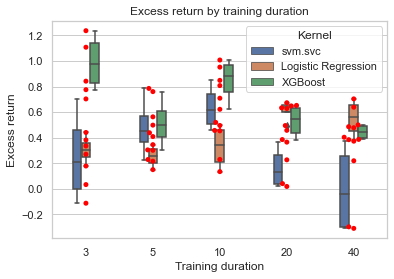
Excess return by training periods

When should we trade our target stock?

If you’re an algo trader who adjusts your portfolio on a daily/weekly/monthly basis, I believe you have the same question as I do: When should I place my order on the day I adjust my portfolio?. The stock prices fluctuate in one intraday. Therefore the timing we place our order could potentially impact our portfolio return.

Here I did a quick experiment by backtesting each scenario two times, one scenario places orders around 09:30 after the market is open, and the other places orders around 14:40 before the market closes. Interestingly, the second scenario has a 77.78% probability to win the first. Meaning, if we place our orders before the market closes, we will have a 77.78% of chance to generate more profit. See the below diagram for the distribution of return differences by models:

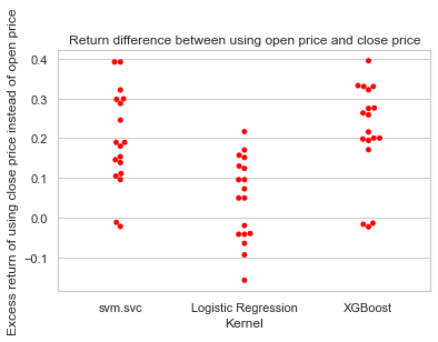
Return difference between placing orders after the market is opened and placing orders before the market closed

There are a few possible reasons I have in mind that might explain why this is happening:

• In the training process, I use close price to label the stocks instead of the open price. So, placing orders before the market closes will help me get closer to the trained model.
• When there’s bad news happening, the stock prices incline to move a lot faster than any other time. Stock prices drop drastically in the pre-market, and will reach our stop -oss point right after the market opened. However, a movement like this tends to bounce back more or less on the same day in the afternoon. So placing orders in the afternoon would prevent us from stopping loss too early.
• A lot of intraday traders and speculators tend to close their positions before the market closes as they have done their work exploiting insider news or any other news. When all the speculations have been digested by the market, the stock price will be much more reasonable and stable.

Is AUC the indicator we use to evaluate our models?

As explained in the above questions, AUC is the indicator to evaluate the accuracy of your classification model. But, does the AUC has a positive relationship with our portfolio return? Let’s first take a look at the regression plot between the AUC and the portfolio return of all our backtest below.

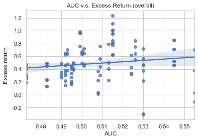
AUC v.s. return

The diagram above doesn’t imply a positive correlation between AUC and portfolio return. The regression slope is quite flat, indicating AUC has a close-to-zero connection with the portfolio return. So it almost is a random walk. No way!! How could weeks of work tell me that this model is useless!?

Calm down. Let me use another angle to diagnose this plot again. I’m adding another dimension to separate the dots by the model we use. Now let’s see how it looks like.

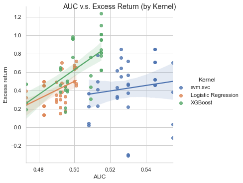
AUC v.s. return(by models)

Wow wow! Now it looks different. The diagram actually tells me that the XGBoost model and the Logistic Regression model contain a certain degree of positive correlation between AUC and portfolio return. This relationship will be buried if we look at each dot is from the identical model.

There are two possible reasons that why the first diagram can’t tell us there’s a potential positive correlation but the second one can:

• The regression was contaminated by the outlier examples lies in the bottom right quadrant.
• We shouldn’t compare AUC across different models.

Before we close this topic

I believe that 108 backtests are actually not enough to help us cover every spectrum in order to answer these questions. However, I think this could be a starting point for you to understand how we can approach these types of questions in order to evaluate the effectiveness of our machine learning trading algorithm.

See you next time.