An investment strategy that takes you three days a year

This is my first article after 2 months of digging, reading, researching, and backtesting. Here I would like to share the result with people who are interested in it and welcome any thoughts from anyone.

Introduction

Before diving into this article, you can start with reading the following thoughts and see whether these are the situations that you’re facing:

My daytime salary is stable, and I want to make some small money by investing in the stock market or ETFs
I don’t have a finance background or experience in putting money in the stock market before
I don’t want to spend too much time and I don’t have enough time to analyze tens of thousands of stocks myself
I know what I should do and how to do it, but buying stocks would literally consume the rest of my day as I don’t want to lose too much money on this.

If you’ve asked these questions to yourself in the middle of the night or during work sometime, this article might help introduce you to some ideas to help you get rid of these thoughts that haunts you.

Background Story (Magic Formula v.s. Acquirer’s Multiple)

The Magic Formula was first introduced in the book “The Little Book that Beats the Market“ by Joel Greenblatt.

The formula is about using ranking of two fundamental stats: Earnings Yield and Return on Capital to quickly identify the value stocks/companies. Once we have our candidates picked, then we buy and hold them for a year and re-evaluate the performance of the portfolio annually. By applying these two numbers as your filters, you’ll be able to locate the stocks/companies that make more money (high Return on Capital, or ROC), but in the meantime is undervalued (high Earnings Yield, or EY).

And then Tobias Carlisle introduced an updated version of the Magic Formula, called Acquirer’s Multiple in his book “The Acquirer’s Multiple“.

As Buffett said, a wonderful company is the one with a high return on equity. The Acquirer’s Multiple uses operating earnings instead of using EBIT. The formula is also inverted. Operating earnings is constructed from the top of the income statement down, whereas EBIT is constructed from the bottom up.

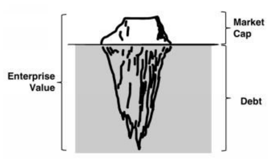
In short, Greenblatt’s Magic Formula is looking for a company that makes money for each dollar that stakeholders invested, while stakeholders pay as little as possible. This is what Buffet has been practicing as he preached over the years. And Tobias’s Acquirer’s Multiple is to find out the company’s cashflow hidden under the iceberg. The lower the Acquirer’s Multiple, the more value you get for the price you pay and the better the stock.

In this article, I’m using Quantopian as the platform for constructing my research and backtesting the strategies to find out the result.

Reference

價值投資者：喬伊‧葛林布雷 (Joel Greenblatt)的神奇公式:『MAGIC FORMULA』 - by 雷浩斯

Greenblatt builds a magic formula on Buffett style ideas - by Robert Abbott

Acquirer’s portfolio year in review - by Ryan Boselo

Magic Formula Strategy in Quantopian - from Quantopian

Comparing the Acquirer’s Multiple to the Magic Formula - from Quantopian

Here comes the Meat!!

Assumptions

Establish a threshold of market capitalization of the company (\$100M~\$1B).
Exclude stocks in the utility and financial sector
Exclude foreign companies ADR (American Depositary Receipts).

Formula

Using Magic Formula
- We’re going to rank both earning yield and roic (the higher the value, the smaller number the rank)
- Add up these two ranks
- We take the top N stocks that rank the highest (top N smaller rank numbers)
Using Acquirer’s Multiple
- We’re going to rank the calculated AM number in reverse order (the lower the value, the smaller number th rank)
- We take the top N stocks that rank the highest (top N smaller rank numbers)

Weight distribution

We are going to test how these three different weight distribution methods impact the return of our portfolio, and find out which one would be better.

Weight evenly
Weight by rank
Weight by Market Cap

Let’s get started

Most research and papers have suggested that owning 25~30 stocks would adequately diversify the sector risk of the portfolio. For individual investors like us, owning that many stocks would be too troublesome. I’m thinking of using 12 as the limit. Also, we’re going to rebalance our portfolio once per year, selling losers one week before the year-mark and winners one week after the year mark. This strategy will need to continue over a long-term period (5~10 years). In this backtest, we’re using 2011/01/01 ~ 2020/07/30 as the backtest period.

How to understand the diagram?

Blue line: returns of the algorithm

Red line: returns of SPY (S&P 500)

Returns: the final return of the algorithm at the end of the backtest date

Alpha: Excess market neutral return that is generated by this strategy

Beta: Represents an individual stock’s returns against those of the market as a whole

Sharpe: How much returns can we get if we take one more unit of risk

Drawdown: Maximum lost in a continuous period

Capacity: Max number of stocks that we’re going to contain in our portfolio

Scenario 1: Buy all and sell all at the beginning of each year

Magic Formula

	Capacity = 12	Capacity = 25
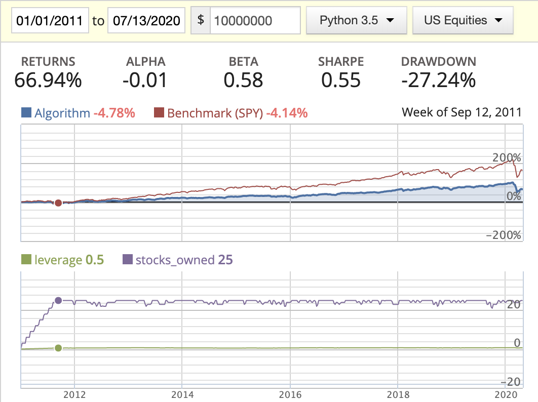
Rank weighted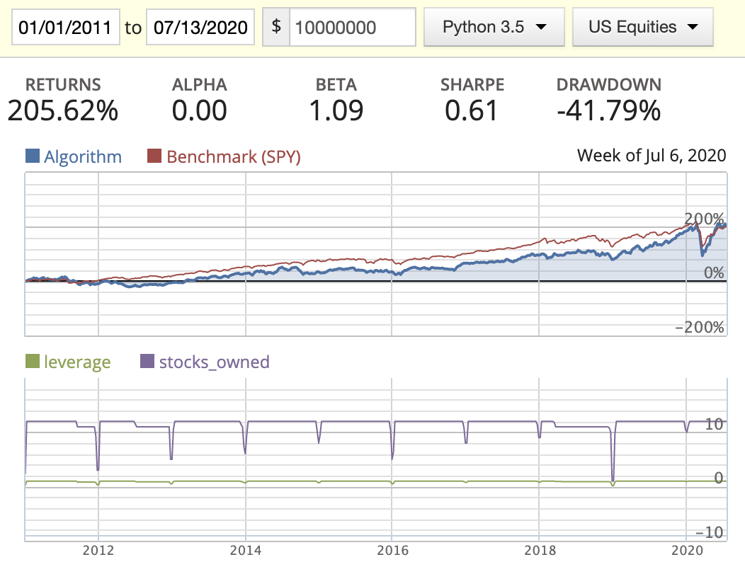
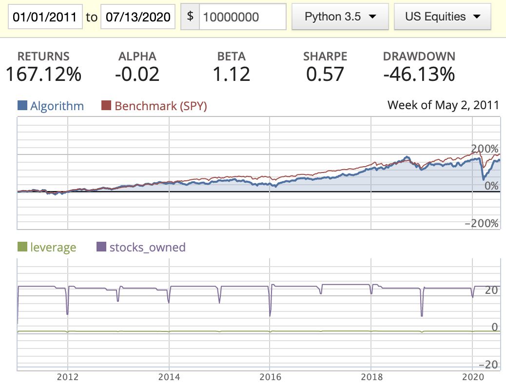
Evenly weighted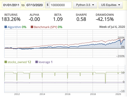
Market cap weighted

Acquirer’s Multiple

	Capacity = 12	Capacity = 25
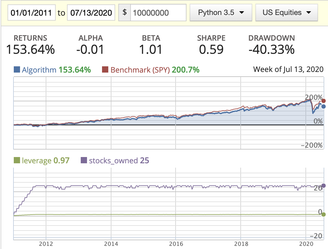
Rank weighted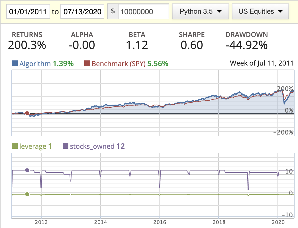
Evenly weighted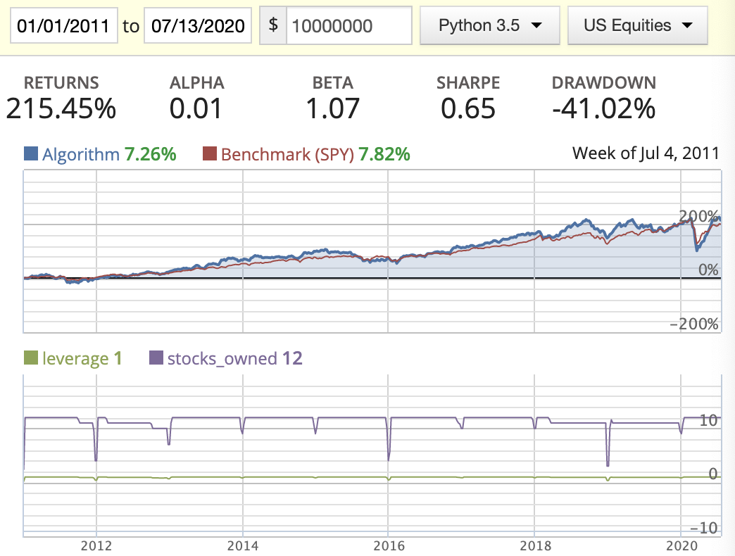
Market cap weighted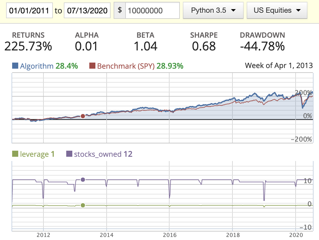

Conclusion

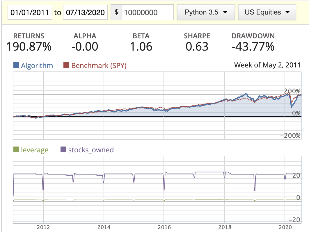
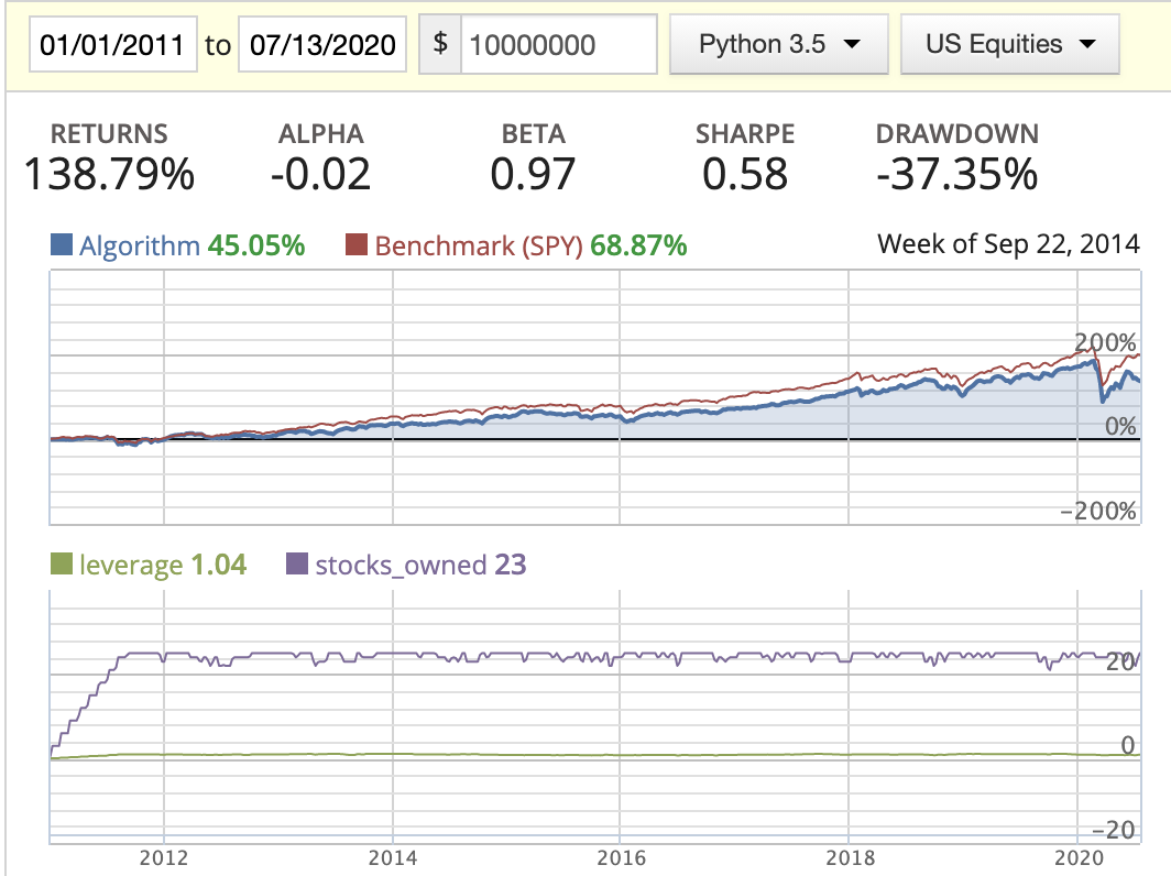
Big capacity doesn’t really imply a well diversified portfolio. You could include a stock that potentially hurts the return of the portfolio.
Seems AM does do better than MF in this scenario.
We can’t tell which weight distribution method is better at the moment.
demean(groupby=Sector()) is a built-in factor function in Quantopian IDE. It deducts the mean of industry sector from each stock, removing part of the differences by sector. In the code we added this function, and it did help improve the performance as it has normalized the Sector risk/exposure.

Scenario 2: Buy all and sell all and use rolling data for the past three quarters

In this scenario, for all the factors such as EV, EBIT, ROIC, …etc, I’m using a three-quarter rolling mean to smooth the data. By doing this, we can mitigate the zig and zag of the quarter numbers and reduce the chances of picking a stock that only stands out in one specific quarter.

Magic Formula

	Capacity = 12	Capacity = 25
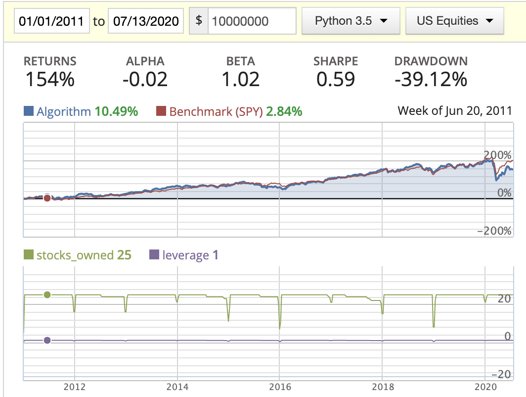
Rank weighted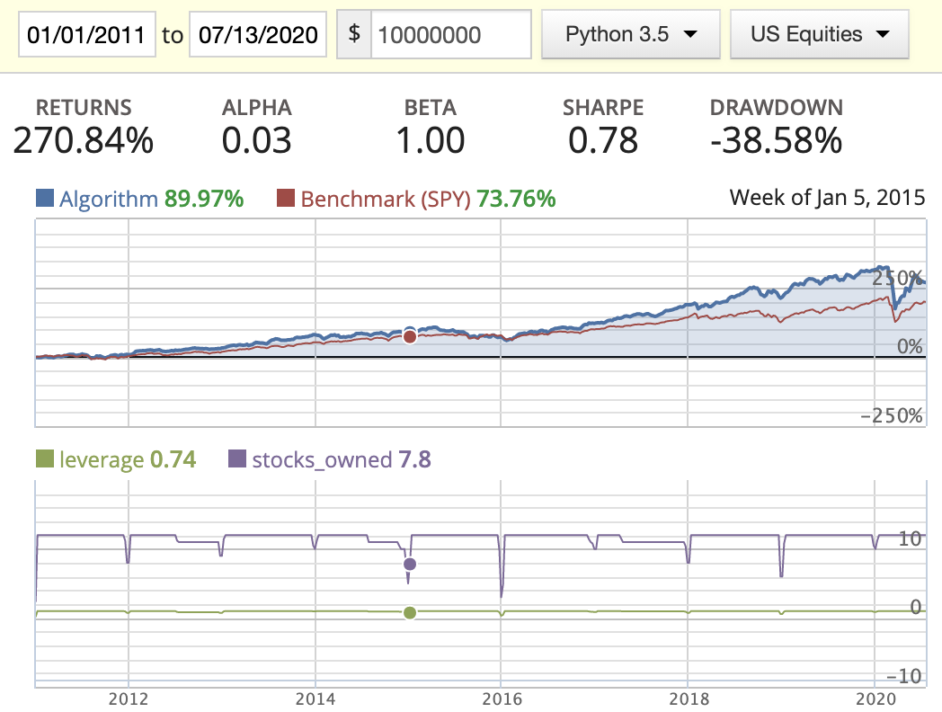
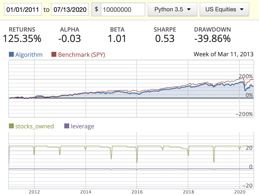
Evenly weighted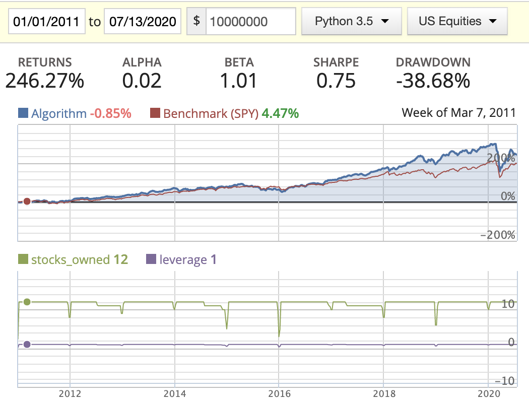
Market cap weighted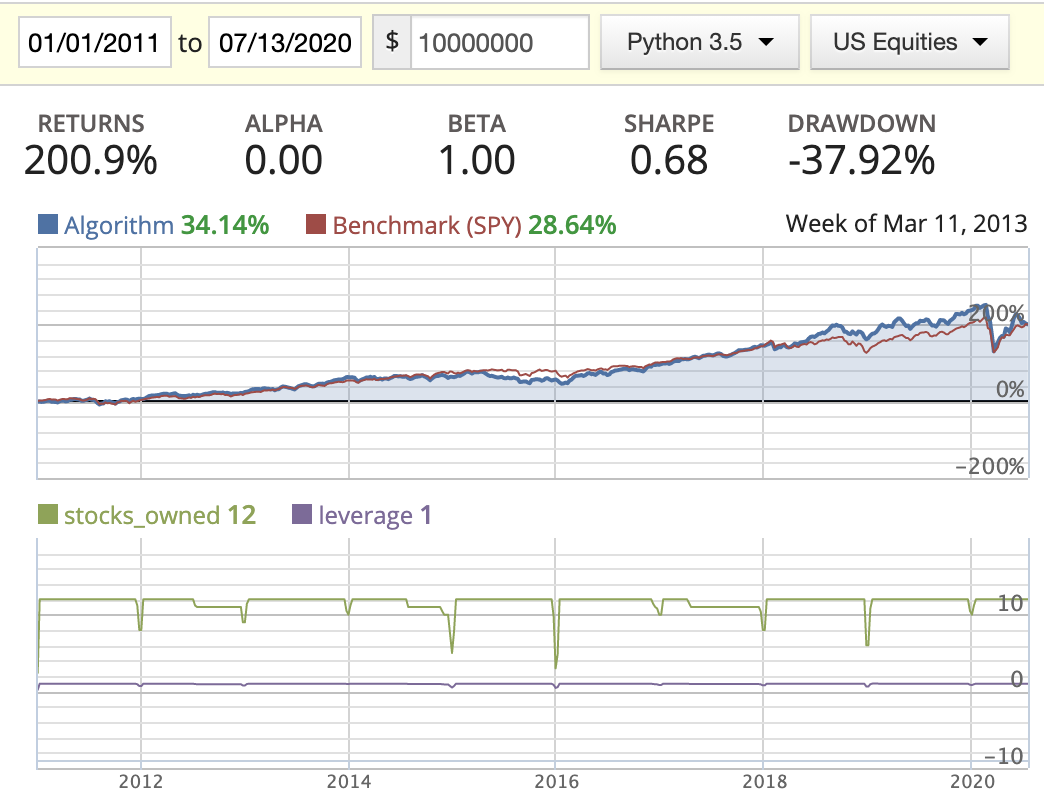

Acquirer’s Multiple

	Capacity = 12	Capacity = 25
Rank weighted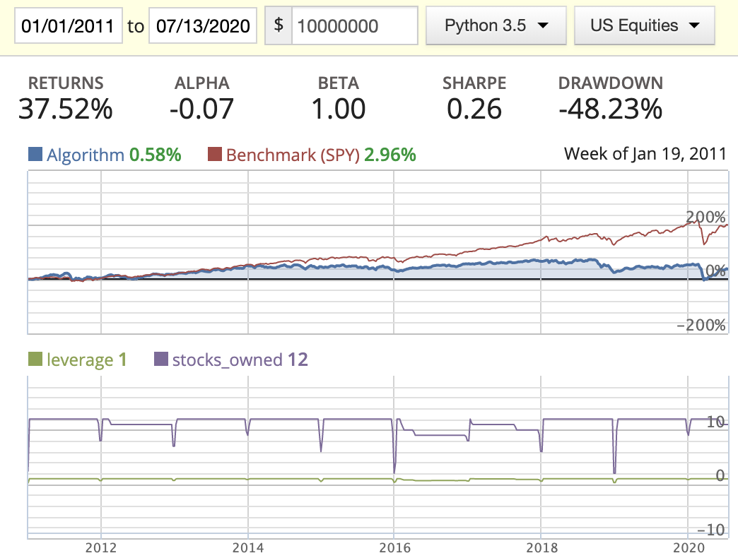
Evenly weighted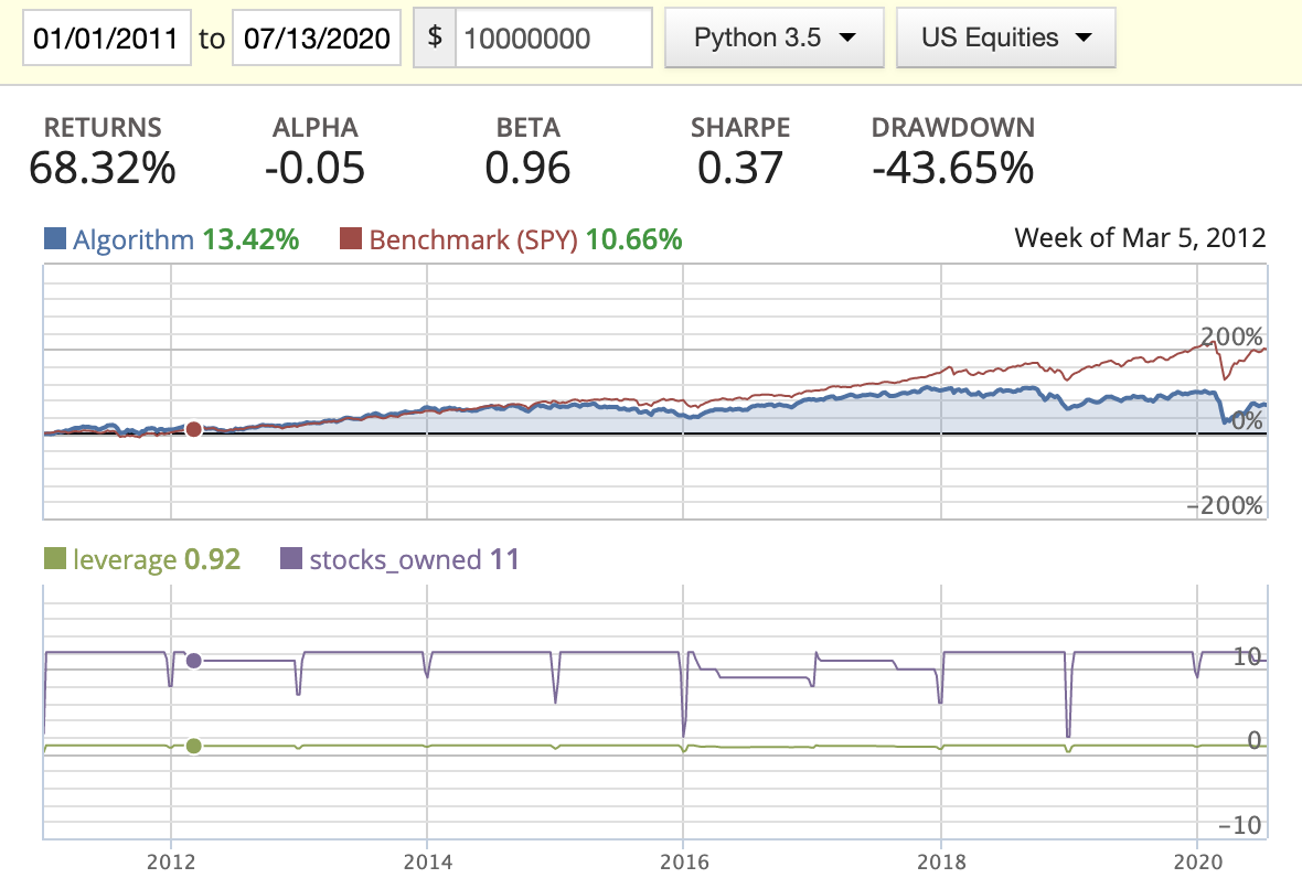
Market cap weighted

Conclusion

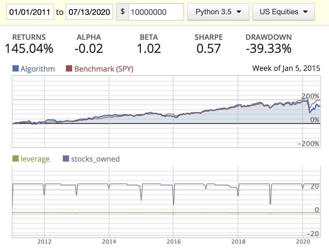
When implementing the rolling rank, I’ve noticed that a lot of stocks are missing EBIT or missing ROIC in their historic data sets, so I dropped those completely. If we had more complete data, the performance of this method might be better.
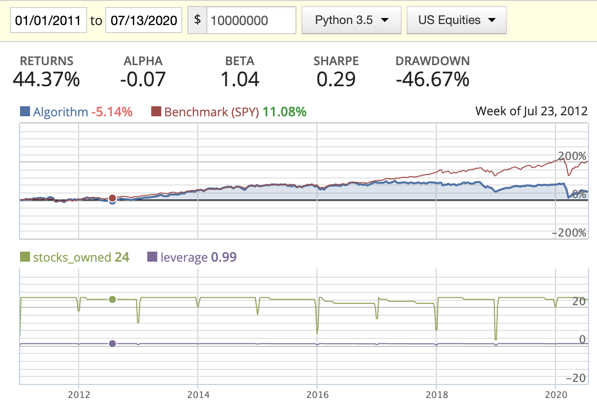
While backtesting using the AM method, we can clearly see the return drastically decrease starting in 2016. By looking at the stocks_owned in the diagrams, you’ll see that three stocks disappeared in the middle of the year. After printing out the owned stocks for each period, we found out that the following three stocks: BMR, SWI, and IRC had either changed their symbol or been delisted from the market, resulting in part of our capital being locked down. I tried to figure out a way to update this in either the log or the portfolio capital, but found that this needs to be managed manually.
Rank weighted distribution is the best option here as it guides us to put more capital in the better quality stocks/companies.

Scenario 3: Buy three stocks maximum per month + Adjust portfolio monthly and use rolling three quarters factors

In this scenario, we re-balance our portfolio on a monthly basis, and buy the top 3 stocks per month in order to make sure we’re able to pick the top ranked stocks. For theMarket Cap-weighted and Rank-weighted method, I discarded them as you need to adjust your positions every month. This also means, that the number of turnovers would increase quite a lot compared to in an evenly-weighted portfolio. I would rather look into this strategy later than now.

Magic Formula

	Capacity = 12	Capacity = 25
Rank weighted (x)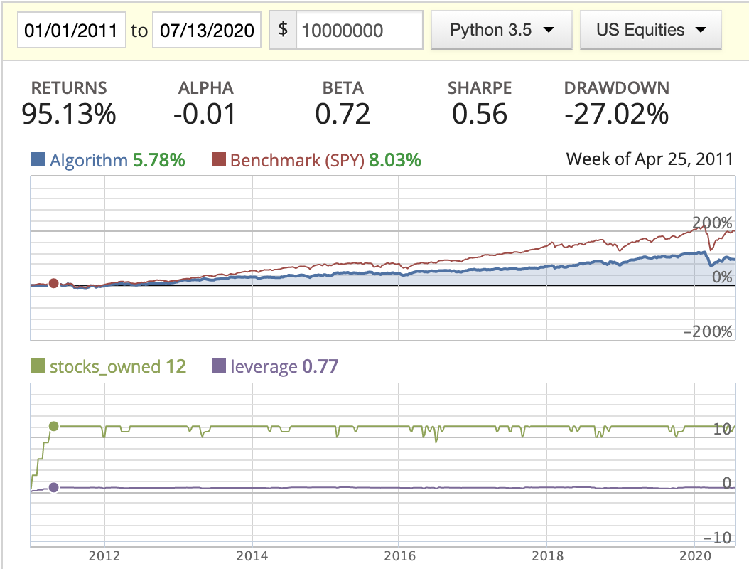
Evenly weighted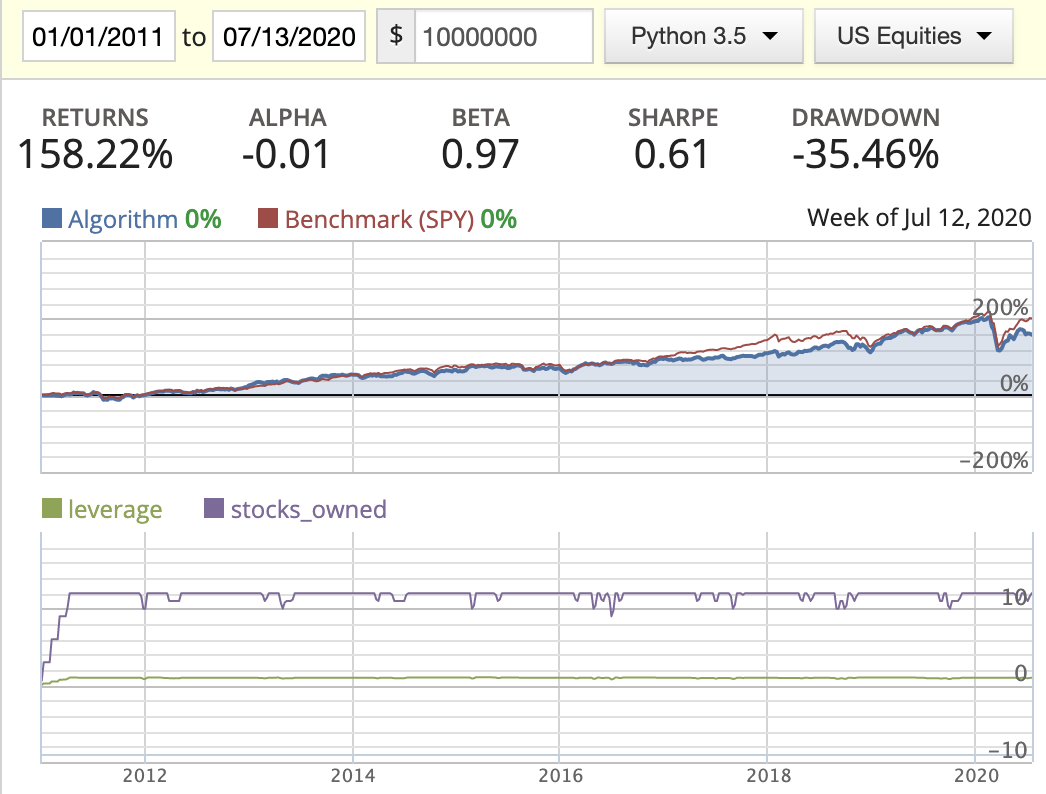
Market cap weighted (x)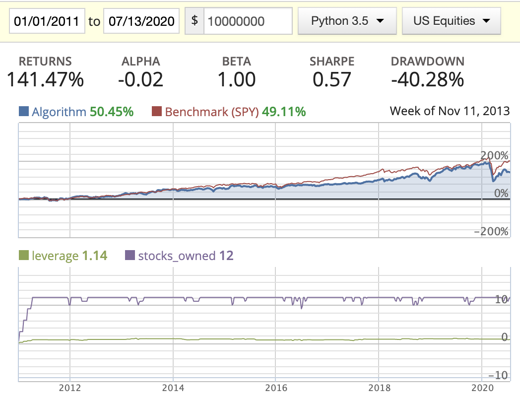

Acquirer’s Multiple

	Capacity = 12	Capacity = 25
Evenly weighted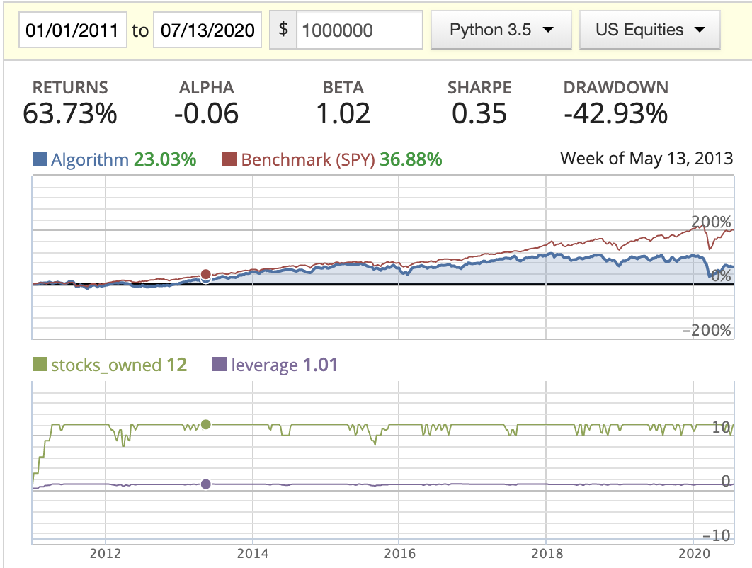

Conclusion

In this scenario, we saw the stocks_owned line has very frequent movement, meaning we’re trading very frequently.

Additional step

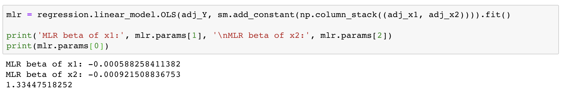
In the magic formula, we’re actually assuming the EY_rank and roic_rank are weighted equally.

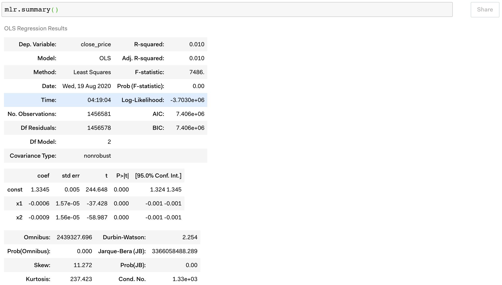
$MF\_rank = 0.5 \times EY\_rank + 0.5 \times roic\_rank$

So what we could do is to use a linear regression to find out the relative coefficient of these two independent variables. Once we have these two coefficients, we can better describe the relation between these variables, and better predict the quality of the company with the Magic Formula.

$MF\_rank = 0.7 \times EY\_rank + 0.3 \times roic\_rank$

However, after performing an OLS linear regression (it’s a basic type of linear regression in the python built-in statsmodels package ) to find out the coefficient of the two independent variables, I found out that the data set is very skewed in terms of the distribution of the daily return of the stock price across stocks. To dive into this topic further, there’re a few more things we can do:

use log return over daily percentage change
Demean the log return by sector

But I’ll leave the thoughts here for now.

Final words

I’ll probably go with the strategy of Scenario 2, 12 assets max, with rank-weighted distribution. The total return has constantly beaten the S&P 500 index over the years covered in the simulation. Also you got an alpha that is positive, a beta slightly over 1, an ok Sharpe ratio, and annual returns around 30% over 8 years. Even when the big slide of COVID-19 hit the market, this strategy still beat the market and was able to rebound quickly enough back to where it was.

“What can I get out of this research and backtesting?” you must be wondering. To answer the questions that we raised in the beginning of the article, I believe this strategy does bring you the benefit that:

We only need to spend 1 morning and 2 evenings in the entire year to complete the trading actions of this Magic Formula strategy.

Doesn’t this sound amazing and attractive!?

Thank you, and let me know if you have any thoughts.

Appendix

Statistics that used in the Magic Formula

息税前利润(EBIT) = 净利润 + 财务费用 + 所得税费用
net_profit 净利润(元)
financial_expense 财务费用(元)
income_tax_expense 所得税费用(元)
固定资产净额(Net Fixed Assets) = 固定资产 - 工程物资 - 在建工程 - 固定资产清理
- fixed_assets 固定资产(元)
- construction_materials 工程物资(元)
- constru_in_process 在建工程(元)
- fixed_assets_liquidation 固定资产清理(元)
净营运资本(Net Working Capital)= 流动资产合计－流动负债合计
- total_current_assets 流动资产合计(元)
- total_current_liability 流动负债合计(元)
企业价值(Enterprise Value) = 总市值 + 负债合计 – 期末现金及现金等价物余额
- market_cap 总市值(亿元)
- total_liability 负债合计(元)
- cash_and_equivalents_at_end 期末现金及现金等价物余额(元)
  Here I also attached the Quantopian code that I used to construct the research this time:

Quantopian code

from quantopian.pipeline.classifiers.fundamentals import Sector
from quantopian.algorithm import attach_pipeline, pipeline_output, get_open_orders
from quantopian.pipeline import Pipeline, CustomFactor
from quantopian.pipeline.filters import QTradableStocksUS
from quantopian.pipeline.filters.morningstar import IsPrimaryShare
from quantopian.pipeline.data import Fundamentals

import pandas as pd
import numpy as np

class RiskAdjValue(CustomFactor):
    """
    RiskAdjValue = Average value of past N quarters' / standard deviation of those values
    """
    num_of_quarter = 3
    window_length = 65 * num_of_quarter
    def compute(self, today, assets, out, value, asof_date):
        # asof_date: shape - (number of window, number of stocks)
        # Example:
        # for datetime 1: ([value of stock A, B, C, ...])
        # for datetime 2: ([value of stock A, B, C, ...])
        # for datetime 3: ([value of stock A, B, C, ...])
        values = value
        for column_ix in range(asof_date.shape[1]):
            _, unique_indices = np.unique(asof_date[:, column_ix], return_index=True)
            quarterly_values = values[unique_indices, column_ix]
            if len(quarterly_values) < self.num_of_quarter:
                quarterly_values = np.hstack([
                    np.repeat([np.nan], self.num_of_quarter - len(quarterly_values)),
                    quarterly_values,
                ])
            out[column_ix] = np.nanmean(quarterly_values[-self.num_of_quarter:]) / np.nanstd(quarterly_values[-self.num_of_quarter:])


def initialize(context):
    # Use below as weight_distribution method. Didn't use Enum as it's not in the quantopian import white list
    # context.weight_distribution = 'RANK_WEIGHTED' | 'EVENLY_WEIGHTED' | 'MARKET_CAP_WEIGHTED'
    context.weight_distribution = 'MARKET_CAP_WEIGHTED'

    # context.formula = 'AM_rank' | 'MF_rank'
    context.formula = 'MF_rank'

    # Max stocks in our portfolio
    context.capacity = 12

    my_pipe = make_pipeline()
    attach_pipeline(my_pipe, 'my_pipeline')

    set_slippage(slippage.FixedSlippage(spread=0.02))
    set_long_only()

    #schedule for buying a week after the year start
    schedule_function(func=buy_stocks,
                      date_rule=date_rules.month_start(4),
                      time_rule=time_rules.market_open())
    #schedule for selling losers a week before the year start
    schedule_function(func=sell_losers,
                      date_rule=date_rules.month_end(4),
                      time_rule=time_rules.market_open())
    #schedule for selling winners on the 7th day of year start
    schedule_function(func=sell_stocks,
                      date_rule=date_rules.month_start(3),
                      time_rule=time_rules.market_close())
    # plot record variables
    schedule_function(func=record_vars,
                      time_rule=time_rules.market_close(),
                      date_rule=date_rules.every_day())

def buy_stocks(context, data):
    today = get_datetime('US/Eastern')
    stocks_owned = sum(1 for stock, position in context.portfolio.positions.items() if position.amount > 0)
    open_orders = get_open_orders()

    if today.month == 1:
        for stock in context.output.index:
            if not data.can_trade(stock) or stock in open_orders:
                print("= %s not tradable or in the open_orders..."%(stock))
                continue
            if stocks_owned >= context.capacity:
                print("= Exceeded the limit")
                return
            # Skip stocks already owned
            if stock in context.portfolio.positions:
                print("= %s is already in the portfolio"%(stock))
                continue

            order_target_percent(stock, context.output.T[stock]['weight'])
            print("+ Buy stocks: %s - weight: %.2f"%(stock, context.output.T[stock]['weight']))

def sell_losers(context, data):
    today = get_datetime('US/Eastern')
    open_orders = get_open_orders()

    if today.month == 12 and context.portfolio.positions_value != 0:
        for stock in context.portfolio.positions:
            if data.can_trade(stock) and stock not in open_orders:
                if context.portfolio.positions[stock].cost_basis > data.current(stock, 'price'):
                    order_target_percent(stock, 0)
                    print("- Sell loser stock: %s"%(stock))
                else:
                    print("= Didn't sell stock: %s"%(stock))
            else:
                print("= %s is already in the portfolio"%(stock))
                print(open_orders)


def sell_stocks(context, data):
    open_orders = get_open_orders()
    today = get_datetime('US/Eastern')

    if today.month == 1:
        for stock in context.portfolio.positions:
            if data.can_trade(stock) and stock not in open_orders:
                order_target_percent(stock, 0)
                print("- Sell winner stock: %s"%(stock))
            else:
                print("= Didn't sell stock: %s"%(stock))


def make_pipeline():
    isPrimaryShare = IsPrimaryShare()

    m &= (Fundamentals.market_cap.latest > 1.00e9)
    m &= (Fundamentals.market_cap.latest < 1.00e10)
    m &= (Fundamentals.country_id.latest.eq('USA'))
    m &= (isPrimaryShare)
    m &= (
        (Fundamentals.morningstar_sector_code.latest != 103) &  # Financial
        (Fundamentals.morningstar_sector_code.latest != 207) &  # Utilities
        (Fundamentals.morningstar_sector_code.latest != 206) &  # Healthcare
        (Fundamentals.morningstar_sector_code.latest != 309) &  # Energy
        (Fundamentals.morningstar_industry_code.latest != 20645020) & # Pharmaceutical Retailers - New
        (Fundamentals.morningstar_industry_code.latest != 20533080) & # Pharmaceutical Retailers - Old
        (Fundamentals.morningstar_industry_code.latest != 10280010) & # Apparel Retail - New
        (Fundamentals.morningstar_industry_code.latest != 10217033) & # Apparel Stores - Old
        (Fundamentals.morningstar_industry_group_code != 10150) & # Metals & Mining - New
        (Fundamentals.morningstar_industry_group_code != 10106) & # Metals & Mining - Old
        (Fundamentals.morningstar_industry_group_code != 10160) & # Coking Coal - New
        (Fundamentals.morningstar_industry_group_code != 10104)   # Coal - Old
    )

    ra_EBIT = RiskAdjValue(
        inputs=[
            Fundamentals.ebit,
            Fundamentals.ebit_asof_date
        ],
        mask=m
    )
    ra_EV = RiskAdjValue(
        inputs=[
            Fundamentals.enterprise_value,
            Fundamentals.enterprise_value_asof_date
        ],
        mask=m
    )
    ra_roic = RiskAdjValue(
        inputs=[
            Fundamentals.roic,
            Fundamentals.roic_asof_date
        ],
        mask=m
    )
    ra_market_cap = RiskAdjValue(
        inputs=[
            Fundamentals.market_cap,
            Fundamentals.market_cap_asof_date
        ],
        mask=m
    )
    ra_cap_exp = RiskAdjValue(
        inputs=[
            Fundamentals.capital_expenditure,
            Fundamentals.capital_expenditure_asof_date
        ],
        mask=m
    )

    # Magic Formula
    earnings_yield = ra_EBIT / ra_EV
    EY_rank   = earnings_yield.rank(ascending=False, mask=m)
    roic_rank = ra_roic       .rank(ascending=False, mask=m)
    MF_rank   = EY_rank + roic_rank

    # Acquirer's Multiple
    ACQ_MULTIPLE = ra_EV / (ra_EBIT + ra_cap_exp)
    AM_rank = ACQ_MULTIPLE.demean(groupby=Sector()).rank(ascending=True)

    return Pipeline(
        columns={
            'ra_roic'       : ra_roic,
            'ra_EBIT'       : ra_EBIT,
            'ra_EV'         : ra_EV,
            'ra_market_cap' : ra_market_cap,
            'MF_rank'       : MF_rank,
            'AM_rank': AM_rank,
            'market_cap': Fundamentals.market_cap.latest,
        },
        screen=m
    )

def before_trading_start(context, data):
    # Trim the output to the picked stocks
    context.output = pipeline_output('my_pipeline').dropna().sort_values(by=context.formula, ascending=True).head(context.capacity)

    if context.weight_distribution == 'EVENLY_WEIGHTED':
        # Weight evenly
        context.output['weight'] = 1.0 / int(context.capacity)
    elif context.weight_distribution == 'RANK_WEIGHTED':
        # weight as rank normalize 0 to 1
        # Weight by rank number
        context.output['weight'] = context.output[context.formula] / context.output[context.formula].sum()
    elif context.weight_distribution == 'MARKET_CAP_WEIGHTED':
        # Weight by market value
        context.output['weight'] = context.output['market_cap'] / context.output['market_cap'].sum()
    else:
        pass

def record_vars(context, data):
    record(leverage=context.account.leverage,
           stocks_owned=len(context.portfolio.positions))